Problems with retrieval
As we have discussed, a sub-optimal retrievers’ embeddings or granularity of data chunks may affect the matching of documents to user queries causing hallucinations in RALMs.
In this section, we will review current methods that address these problems.
In search of optimal embeddings
A standard embedding model learns query and text representations using an encoder-based architecture (e.g. BERT and RoBERTa). To learn such representations, practitioners usually fine-tune pre-trained embeddings with a loss function that contrasts a positive query-document pair against random negative pairs. Such pairs are usually sourced from textual entailment texts from heterogeneous set of publicly available letters, reports and articles resulting in general-purpose embeddings.
While working well for those RALMs that utilize standard external databases like Wikipedia, such general-purpose embeddings often perform poorly in new domains that are often encountered in medical and financial applications. For example, retrieval performance of BERT’s embeddings in this Massive Text Embedding Benchmark drops from 61% to 15% when changing Quora-based dataset to dataset dedicated to COVID-19.
Synthetic data for fine-tuning
Experience from other tasks in natural language processing suggests that fine-tuning text-embeddings on the data from the domain of interest can improve RALM’s performance in that domain. However, finding a fine-tuning dataset is not easy. Unlike pre-training data for masked language modelling, fine-tuning datasets for RALM require annotations (samples in these datasets must include {query, response, relevant documents} triplets). This poses a challenge in new domains that are quite specific (e.g. subfields of law or finance) and have little or no annotated data. For such domains, apart from annotation of query-response-documents triplets, finding a relevant knowledge corpus of the size large enough (usually 50k - 250k documents RAG-studio, Query reconstruction) can already be a problem.
One way to sidestep this is to use language model to generate a synthetic fine-tuning data.
Following this direction, authors of [RAG-studio] propose a two-stage approach. First, using a general-purpose retriever and language model they create a synthetic fine-tuning dataset based on unlabelled data from the domain of interest. Second, after applying several filtering heuristics they fine-tune the initial retriever on this data to adapt it to the new domain. As a result, their method outperforms even the baseline that used non-synthetic fine-tuning data in Biomedical, Financial, and Legal domains. Below, we provide more details on their synthetic dataset creation and retriever fine-tuning.
Raw synthetic dataset creation
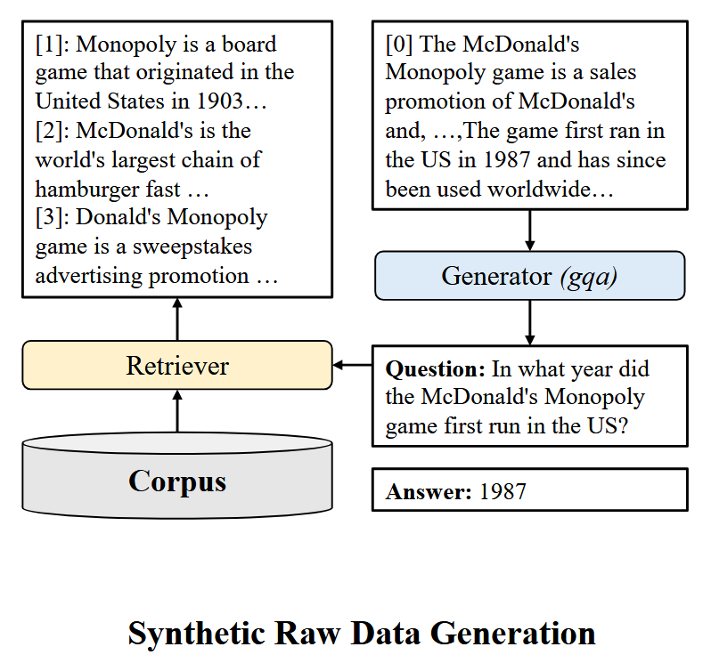
The input to RAG-Studio includes a domain corpus with multiple documents $\mathcal{D} = \{c_1, \ldots, c_n\}~,$ a general LLM-based generator $G$, and a retriever $R$. First, a generator $G$ is prompted to produce a query $x$ and its corresponding response $y$ based on a ground document $c_{\text{gold}}$ which is randomly selected from $\mathcal{D}$ (by design this document will be the most relevant “golden” context for the produced query):
\[x, y = G\left( \begin{aligned} \text{"Generate query and response pair, such} \\ \text{that response is based on \{c_{gold}\}"} \end{aligned} \right)\]Note: The prompts in this section are not exactly the same as those in the paper. They are provided to give a high-level understanding.
Next, to provide additional context, the authors retrieve the top-K documents from $\mathcal{D}$ for the generated query (the document $c_{\text{gold}}$ is excluded from the results):
\[c_1, \ldots, c_K=R(x, \mathcal{D})\]This results in synthetic raw training samples of the following form:
\[s=\left(x, y, c_{\text{gold}},\left\{c_1, \ldots, c_K\right\}\right)\]The figure below shows an example of raw synthetic dataset creation. The ground document $c_{\text{gold}}$ (starting with “[0]”) is given to generator to come up with query $x$ (question starting with “question: In what year ….”) and response $y$ (answer 1987) pair. Then the question is used to extract additional documents $c_1, \ldots, c_K$ (documents starting with “[1]”, “[2]” and “[3]”).
Positive and negative pairs for retriever
Similarly to popular techniques, the retriever is fine-tuned using a loss that contrasts positive query-document pairs with random hard negative pairs. The mining process for such pairs is divided into two stages.
In the first stage, the generative model answers the question with a chain-of-thought reasoning. During this reasoning the model evaluates and classifies each context document into one of three categories: “helpful”, “irrelevant”, or “misleading”. The final answer is then generated based on this evaluation. The whole process can be expressed as follows:
\[H^{\prime}, y^{\prime}= \left( \begin{aligned} \text{"Evaluate how helpful each document in \{C\} is for answering \{x\}.} \\ \text{Use this reasoning to answer the question."} \end{aligned} \right)\]Where $C = \{c_1, \ldots, c_K\} \cup c_{\text{gold}}$ or $C = \{c_1, \ldots, c_K\}$, $y^\prime$ is predicted response and $H^{\prime} = h^{\prime}_1, \ldots, h^{\prime}_K$ contains helpfulness labels $h^{\prime}_i$ $\{\text{“helpful”, “irrelevant”, “misleading”}\}$ for each document in $C$ and chain-of-thought rationale for these labels.
An illustration of the first stage is shown in the figure below. The generator receives a set of retrieved documents (starting with “[1]”, “[2]”, and “[3]”) along with a question from the previous figure (starting with “Question: In what year …”.). It then generates an answer (1903, which is incorrect since 1987 is the correct answer for the current question, as can be seen in the previous figure) and a rationale that evaluates the helpfulness of each document (starting with “[Evaluation]: [0] discusses.…”). Finally, it assigns helpfulness labels to each retrieved document ([helpful, helpful, irrelevant, misleading]).
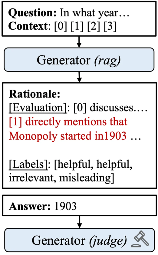
In the second stage, the generator’s predictions $H^{\prime}$ and $y^{\prime}$ are used to provide positive and hard negative signals for the retriever’s contrastive training. Namely, when $y^{\prime}$ is correct, documents marked as “helpful” are treated as positive samples while documents marked as “misleading” are treated as hard negatives for the question $x$. Inversely, when $y^{\prime}$ is incorrect, “helpful” documents are considered as hard negatives. In both cases the original ground document $c_{\text{gold}}$ is treated as a positive sample.
This process is illustrated in the figure below. The original ground document $c_{\text{gold}}$ (starting with “[0]”) is treated as a positive example. Document $c_1$ (starting with “[1]”) is originally labeled as “helpful”, and therefore, is treated as a hard negative example. This is because the answer predicted by generator (1903) was incorrect, as shown in the previous figure.
Contrastive loss for retriever
After collecting the positive documents $C^{+} \in \mathcal{D}$ and the hard negative documents $C^{-} \in \mathcal{D}$ for the query $x$ from the helpfulness rationale of the generator $H^{\prime}$, the authors employ the contrastive ranking loss function to fine-tune the dense retriever by aligning it with the generator’s preference:
\[\mathcal{L}_{\mathrm{C}}=-\log \frac{p(c^{+} \mid x)}{p(c^{+} \mid x)+\sum_{c^{-} \in C^{-}} p(c^{-} \mid x)}\]where $p(c \mid x)$ is the the retriever’s probability to extract document $c$ from $\mathcal{D}$ given a query $x$.
Joint fine-tuning of retriever and generator
In the previous section the retriever was fine-tuned on synthetic data independently of the generator. Since the final goal of fine-tuning is to make sure that RALM not only uses relevant documents but also produces desirable responses, it is reasonable to fine-tune the retriever with supervision on expected responses, in addition to retrieved documents.
One way to capitalize on this idea and adapt retriever’s embeddings to new domains is to fine-tune them jointly with a generative language model (LM) on the available realistic or synthetic data from the domain of interest. Usually, it is done by minimizing the negative log likelihood of the correct response conditioned on the retrieved document.
Let’s denote $p(y \mid c, x)$ as the language model’s likelihood of generating response $y$, based on query $x$, and the retrieved document $c$. The term $p(c \mid x)$ as the probability of a retriever to extract a document $c$ from an external database $\mathcal{D}$. The terms
\[\mathrm{E}_{\mathrm{document}}\text{ and }\mathrm{E}_{query}\]as text encoders that compute embeddings for documents and queries, respectively and can share the same weights.
Then the loss for joint fine-tuning of retriever and generator can be expressed as follows:
\[\mathcal{L} = - \operatorname{log} [ p(y \mid x)]=- \operatorname{log}[\sum_{c \in \mathcal{D}} p(y \mid c, x) p(c \mid x)]\] \[p(c \mid x) =\frac{\exp f(x, c)}{\sum_{c^{\prime}} \exp f\left(x, c^{\prime}\right)}\] \[f(x, c) =\operatorname{E}_{\text{query}}(x) \text { E }_{\text{document}}(c)^{\top}\]Note: we treat embeddings as row-vectors, that is why the dot-product
\[\operatorname{E}_{\text{query}}(x) \text { E }_{\text{document}}(c)^{\top}\]has transpose sign after the second term and not the first.
Reconstruction signal
While the loss above is mathematically sound and widely adopted, in principle its optimization might result in undesirable behaviour when generator learns to ignore all the retrieved documents and predict response based solely on the query. Such an “ignorance” might emerge when the external database contains many noisy or irrelevant documents.
To avoid such trivial solutions and help the RALM adapt to domain-specific knowledge base, the authors of Query reconstruction suggested adding query reconstruction loss as an auxiliary signal to the loss above while fine-tuning their retriever and generator.
They first instruct the retriever to extract documents similar to the user query from the external knowledge base. Then they train the language model to reconstruct the user query using only the retrieved documents.
To help the model distinguish the reconstruction task from the standard task (e.g. QA task), the query $x$ is replaced with the utility token $\text{<p>}$ while expected response $y$ is replaced by the query $x$ itself. After these changes, the training loss is updated as follows:
\[\mathcal{L} =- \operatorname{log}\left[\sum_{c \in \mathcal{D}} p(x \mid c, \text{<p>}) p(c \mid x)\right]\]This loss ensures that when the language model is prompted with $\text{<p>}$ and $c$, it generates such a query $x$, that leads the retriever to extract documents $c$ from the external database.
Note: When the final loss is computed, this auxiliary loss is summed with the main loss from the previous section.
In search of optimal granularity
Another reason for poor retriever performance is the length-unconstrained nature of knowledge sources. For example, converting entire webpages or books into a single document often results in lengthy knowledge database entries.
As we can remember, Large Language Models (LLMs) struggle with processing long documents due to limited context length. Therefore, chunking is a crucial step in retrieval-augmented generation (RAG). It divides long documents into smaller, manageable parts to provide accurate and relevant evidence for generator. Chunking granularity can vary from documents to paragraphs or even sentences depending on the task and knowledge database.
The inevitable question that arises at this point is: how to select the appropriate granularity for the given task?
Too coarse chunking with longer contexts can offer a broader overview but may include irrelevant details that distract LLMs. Too fine-grained chunking provides precise information but risks being incomplete and lacking context.
One simple approach that is widely used in RAG systems is a fixed-size chunking. It breaks documents into chunks of a fixed length, such as 100 words. While this approach benefits from simplicity and universality, it often fails to preserve semantic integrity, structure and dependencies of original long documents and as a consequence affects the relevance of retrieved information.
Splitting into propositions
One way to go beyond fixed-size chunking is to split long documents into smaller texts using another LLM. Following this direction the authors of Dense X Retrieval suggest preprocessing all documents with a summarization model called “propositionizer” and split them into small atomic expressions with a fixed maximum length that encapsulate distinct facts in a concise and self-contained format called “propositions”.
The figure below shows an example of extracting propositions from a document. Given a text about the Pisa Tower, the propositionizer extracts three separate propositions and adds them to the knowledge base.
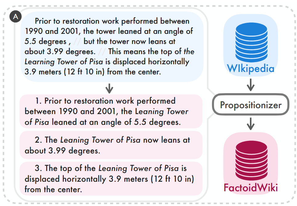
As a result, splitting texts into propositions improves retrieval performance compared to splitting into passages or sentences. For example, the Recall@5 metric (percentage of questions for which the correct answer is found within the top-5 retrieved passages) for the Contreiver retriever increases from 43.0% for passages and 47.3% for sentences to 52.7% for propositions.
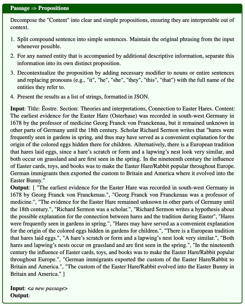
Training a propositionizer model
The Propositionizer is trained using a two-step distillation process. First, the authors prompt chatGPT-4 with an instruction. The prompt includes the definition of a proposition and a one-shot demonstration. They use 42,000 passages and let chatGPT-4 generate a seed set of paragraph-to-proposition pairs. Next, the authors use this seed set to fine-tune a Flan-T5-large model. The figure below shows the details of the prompt shown to GPT-4:
Incorporating documents in a tree-structure
While the previous approach works pretty well, it modifies the original documents with an LLM which might lead to the loss of information.
Therefore, now we will consider the RAPTOR method that allows to keep the original documents intact. This approach also utilizes a separate summarisation model to add additional structure to the database, however, in contrast to the previous approach it extends the database with synthetically generated documents without substituting any initial text chunks.
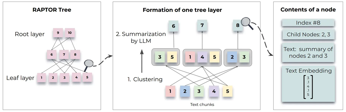
It aims to construct such a tree-structure where higher nodes summarise lower-layer nodes, while the leaves represent the original text chunks obtained by fixed-size chunking. It mitigates the possible issues that arise during initial chunking as the higher-level nodes retain the key details from their child nodes, even if individual leaf-nodes suffer from lost or redundant information.
To build such a tree-structure, RAPTOR first clusters original text chunks using Gaussian Mixture Models. Then it generates text summaries for each cluster, so that each summary becomes a higher node in the tree while all documents in the cluster serve as its children. It repeats the process to build a tree from the bottom up. This whole process can be seen in the figure below:
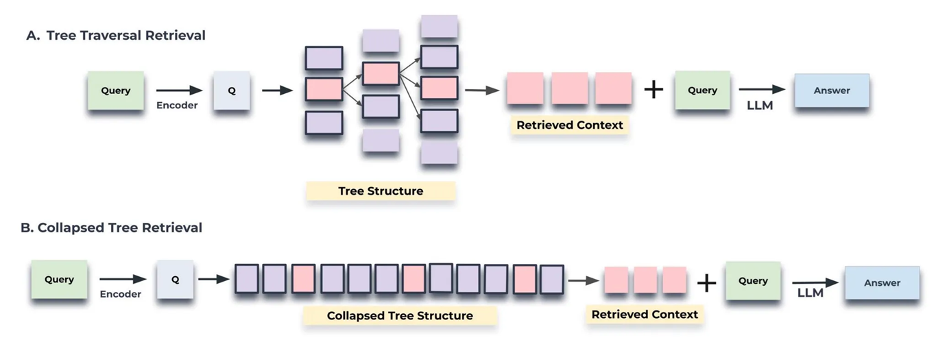
For retrieving documents from this tree, they propose two strategies: tree traversal and collapsed tree. Tree traversal examines each layer one by one from the top to bottom and selects the most relevant nodes. Collapsed tree considers nodes from all layers at once to find the most relevant ones. Relevant nodes are those with embeddings most similar to the query embeddings. The figure below visualizes the tree traversal strategy:
Such a tree structure allows RAPTOR paired with retriever to load chunks into an LLM’s context at different levels, enabling efficient and effective question answering. For example when using RAPTOR in combination with SBERT retriever on QuALITY dataset, accuracy of answers grows from 54.9% to 56.6%.