By: Sergei Skvortsov
Up to this point, it’s natural to wonder: How can I ensure I’m getting the most out of my LLM developments? In this long read, we’ll unpack the core ideas behind inference — including its metrics and mathematical foundations — that are key to optimizing performance. With this understanding, you’ll be better prepared to make smart decisions about deployment strategies, resource optimization, and system design.
The plan is:
-
Inference Essentials. In this section, we’ll discuss key concepts of LLM inference and working with GPUs.
-
Inference Metrics. In this section, we’ll discuss latency and throughput and finding balance between them.
-
Inference Math. In this section, we’ll use our knowledge of transformer architectures to determine the optimal batch size for inference, taking Llama-3.1-8B as our example. We anticipate our findings will be quite surprising!
Inference Essentials
In the context of LLMs, inference is the process where the model takes in a given input (like a sentence or a question) and generates an output (like a response or a continuation of the text). It relies heavily on GPU acceleration and many optimization tricks to handle the intensive computations. Inference should be distinguished from training - during inference we don’t update weights and, in particular, don’t need gradients.
In Topic 4, we discuss how inference operates and what are potential bottlenecks. In Topic 5, we’ll be covering optimizations that make inference more efficient.
Inference Process
Here is a schematic overview of the LLM inference steps:
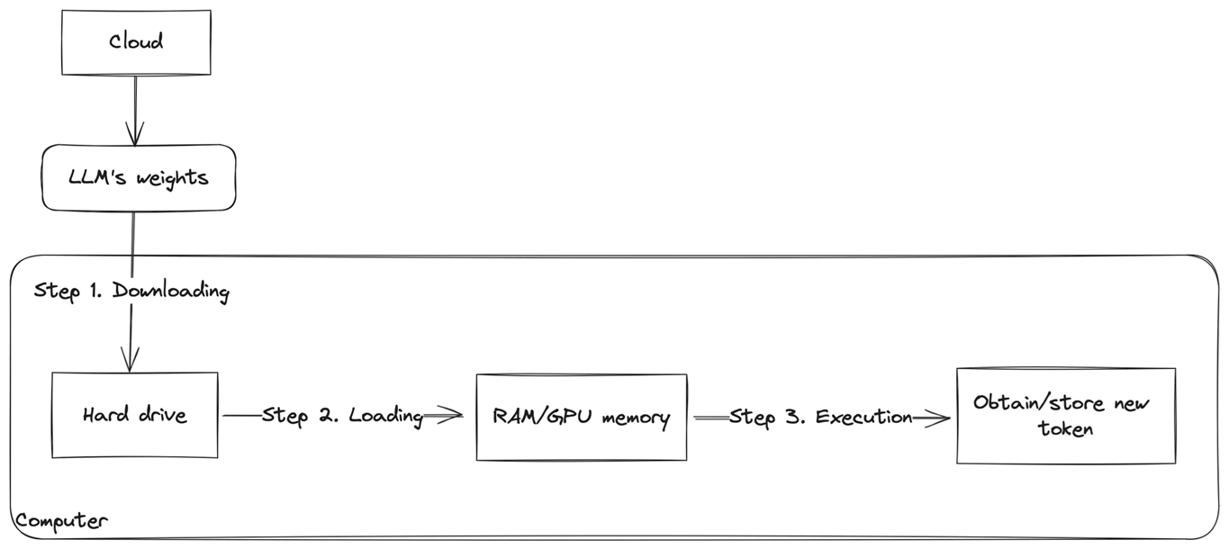
There are three key steps:
- Downloading: This stage involves downloading the model weights, typically from a cloud storage service like Hugging Face. These weights are then stored on the computer’s disk where you plan to run the LLM, whether on a local machine or a remote server.
- Loading: In this step, the LLM’s weights are loaded into RAM or the memory of a hardware accelerator (such as GPU or TPU), preparing the model for generating new token. GPUs and TPUs are predominantly used for modern LLMs due to their superior performance in comparison to CPUs.
- Generation: Finally, the model is ready to generate new tokens. As tokens are generated, they are concatenated into the output sequence, which is returned as the result of the inference process.
Important note: During inference, the model’s weights are not updated; they remain unchanged.
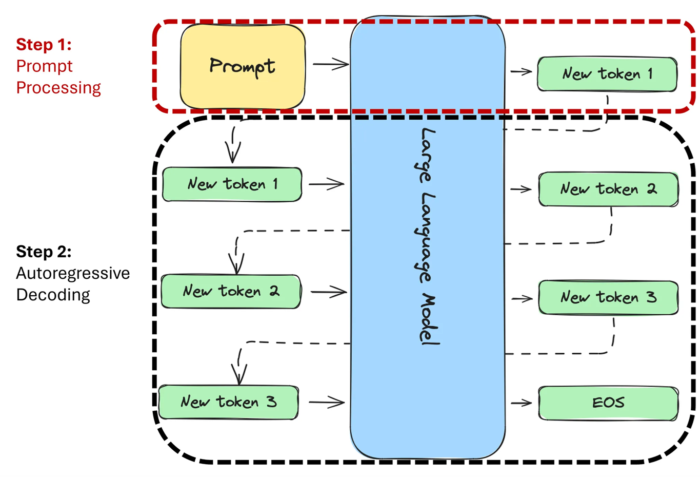
During the generation step, we can distinguish two stages:
-
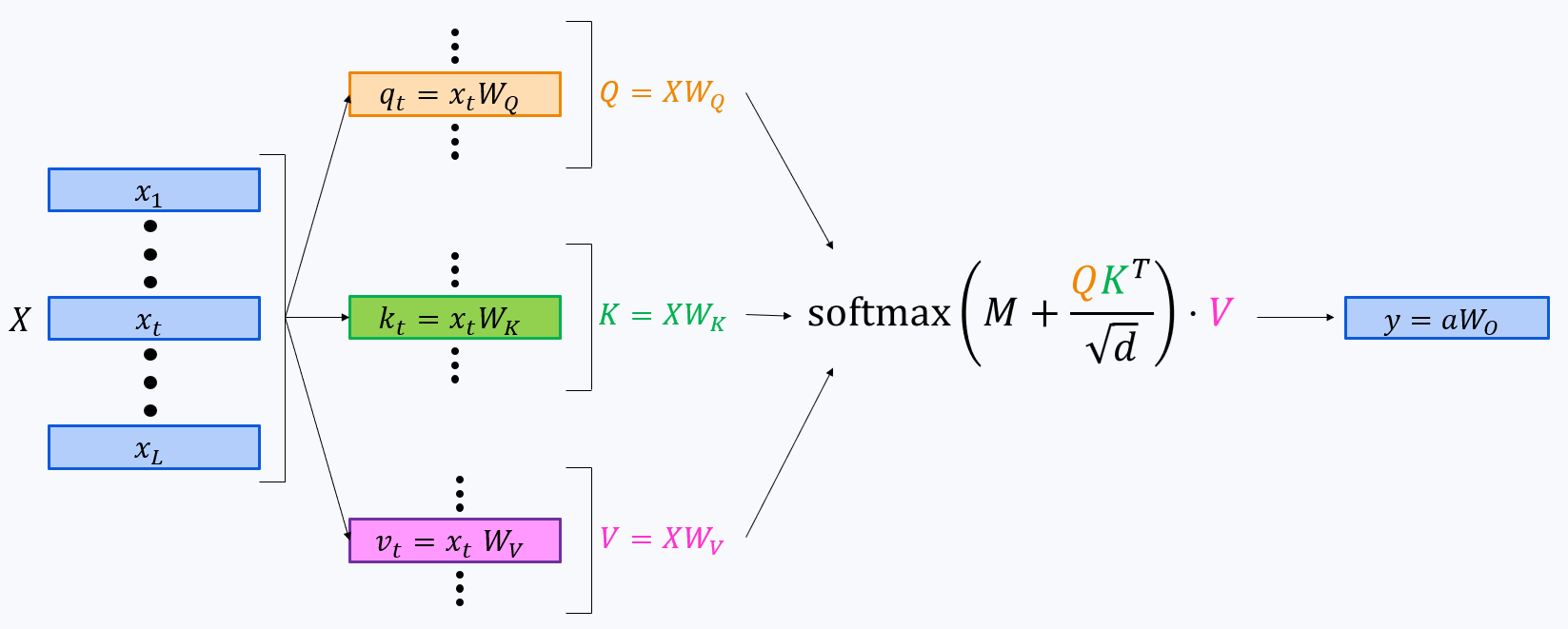
Prompt processing: In this stage, the LLM processes the prompt. When we introduced transformer architecture, we mentioned that self-attention mechanism allows each token to “look” at previous tokens, transforming their internal representations. While this remains true, we can optimize this process for an input sequence by performing these “looks” simultaneously, making it faster (though still quadratic in complexity).
Prompt processing results in the generation of the first token in the output sequence (New token 1).
-
Autoregressive decoding: In the second stage, the LLM generates new tokens autoregressively. This means tokens are generated one by one. To generate the (N+2)-th token, the model must first “look” at the (N+1)-th token (and all the previous ones). This process cannot be parallelized, so each token is computed sequentially. The decoding continues until either an End Of Sequence (EOS) token is generated or the maximum sequence length is reached.
Processing Inference at GPUs
In LLM inference (as everywhere in Deep Learning), GPUs play a critical role by parallelizing tasks, enabling faster computations and efficient resource utilization.
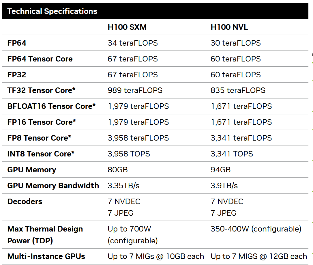
When examining any GPU specific hardware specifications, you’ll notice a variety of different parameters. For instance, you can find the specifications for the H100 GPU on Nvidia’s official website: link
Let’s take a closer look at these parameters:
For our purposes, we need to focus on the following:
-
Peak FLOPS: This refers to how many floating-point operations (such as multiplication and addition) the GPU can perform per second. These values can vary depending on the precision of the model’s weights, meaning how many bits are used to store each parameter.
For inference, FLOAT16 (FP16) or BFLOAT16 (BF16) are commonly used, which are formats for storing floating-point numbers in 16 bits of memory.
For the H100 GPU, the peak FLOPS for FP16 and BF16 is 1,979 or 1,671 teraFLOPS depending on the configuration. Nebius serves H100 NVL, so we will use this number in further calculations.
- GPU memory size: This is the total amount of memory available on the GPU. For the H100, depending on the model, it can be either 80 GB or 94 GB.
- GPU memory bandwidth: This is the maximum speed at which data can be transferred between the compute engine (or CUDA cores) and the GPU memory. It determines how quickly data can be loaded or stored during computation.
To understand these parameters better, let’s explore how a modern GPU works using a simple analogy. There is an excellent article called Making Deep Learning Go Brrrr From First Principles, where the author explains that a modern GPU can be compared to a factory.
To produce goods, raw materials must be transported from a warehouse (GPU memory) to the factory (compute). The speed at which these materials are delivered from the warehouse to the factory is determined by the memory bandwidth. Once the factory receives the materials and processes them (i.e., performs computations, ideally at maximum Peak FLOPS), the results are then transported back to the warehouse (GPU memory).
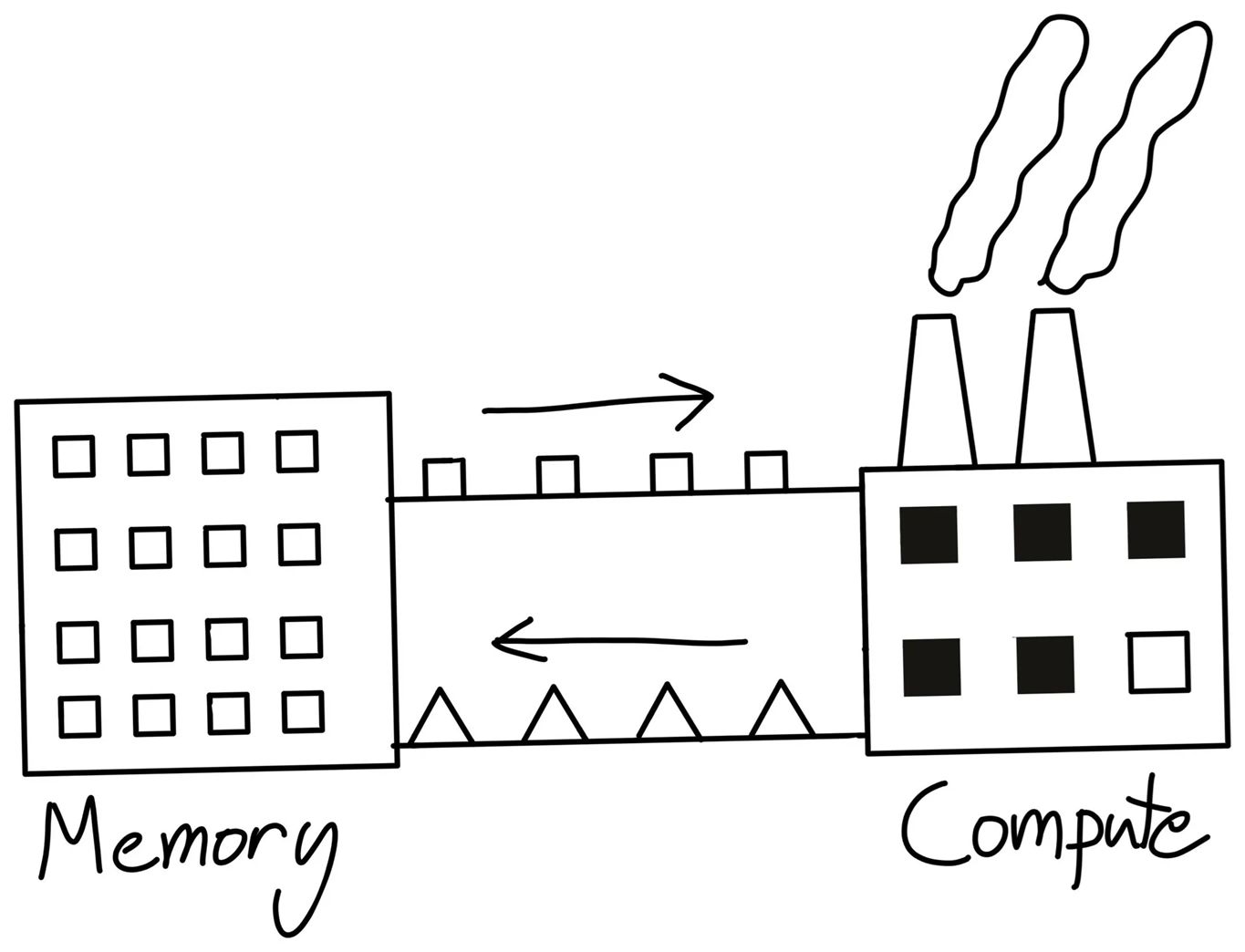
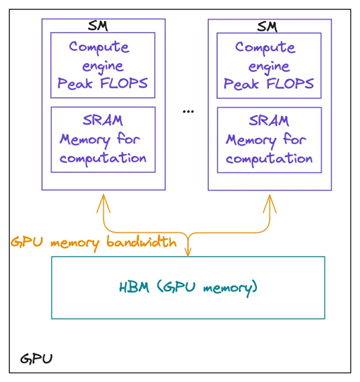
Keeping this in mind, let’s return to how GPUs work. A typical GPU consists of GPU memory (or HBM) and multiple streaming multiprocessors (SMs). An SM is like a large furnace with small local storage and several conveyor belts or furnaces (CUDA cores) that can work simultaneously, but should all perform the same computation. Once the factory receives the materials, it distributes them to its furnaces which process them in parallel.
To perform operations, data must first be loaded from the GPU memory (turquoise colour) into the local memory (or SRAM) of each SM (purple colour) at the speed determined by the GPU memory bandwidth (orange). Then, all compute engines (or CUDA cores) within the SMs process the data simultaneously. Once the computation is complete, the results are stored back in the GPU memory.
It’s important to note that to achieve peak FLOPS, the operation must fully utilise all compute engines on the GPU.
Inference metrics
Evaluating inference is crucial for understanding how LLMs perform in your scenarios and for guiding their optimization. It helps identify performance bottlenecks, manage trade-offs, and adapt models to meet specific requirements for speed, scale, and cost.
Inference Metrics Overview
There are three important metrics:
Throughput: This refers to the number of requests or tokens an LLM can process per second. Increasing throughput allows the system to handle more tokens and requests in the same amount of time, improving overall efficiency.
Latency: This is the time elapsed from when a user makes a request until the LLM provides a response. This metric is especially critical in real-time and interactive applications, such as chatbots and real-time systems, where quick response times are crucial.
Cost: This represents the amount of money spent to process a request. Reducing costs is a common goal, and one way to achieve this is by deploying your own LLM, which you can optimize to lower expenses compared to using third-party services.
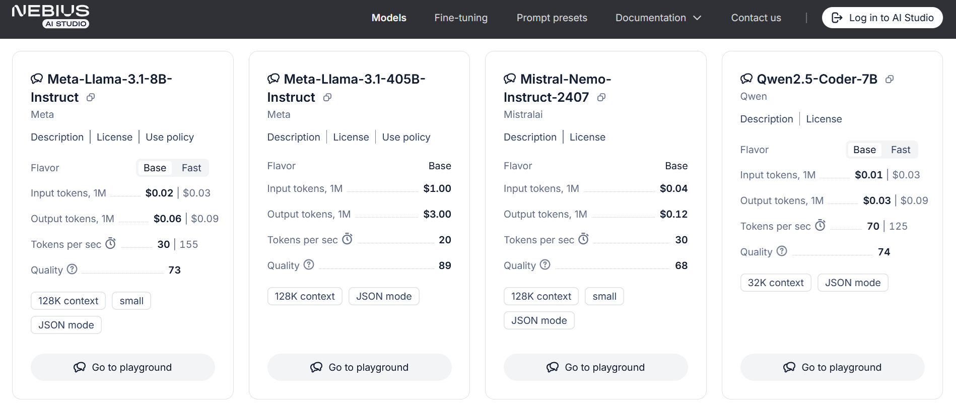
When considering the cost of using LLM inference services (for example, Nebius AI: https://studio.nebius.ai), you’ll notice that input tokens typically cost about three times less than output tokens. As discussed earlier, this difference arises because:
- Processing input tokens generally requires one optimized (although quadratic) pass through the LLM, whereas
- Generating output tokens involves multiple passes — one for each token produced. This increased computational demand for generating output is the reason output tokens cost more than input tokens.
Memory-bound and Compute-bound Programs
Distinguishing between memory-bound and compute-bound programs is crucial for interpreting inference metrics and optimizing LLM performance. These classifications describe whether a model’s performance is limited by memory access speeds or computational power, directly influencing key metrics like throughput, latency, and cost. Therefore, linking these concepts to inference metrics provides deeper insights into how resource utilization and workload dynamics shape the performance of large language models, enabling more effective optimization strategies.
The main difference between these two types of programs is as follows:
-
Compute-bound program: Its execution time mostly depends on the time spent on calculations. A good example of a compute-bound program is matrix multiplication, which requires intensive mathematical calculations.
One way to speed up this type of program is by increasing the speed of the compute engine.
In our factory metaphor, this would be a factory where raw material is processed more slowly than it can be transported from the warehouse.
-
Memory-bound program: Its execution time primarily depends on the speed of data movement. An example of a memory-bound program is matrix transpose. This task involves loading the data into the compute engine, transposing it, and saving it back to memory. Since transposition is a very simple calculation, the operation’s total time is dominated by the time it takes to move the matrix in and out of memory.
Enhancing performance for memory-bound programs typically involves increasing memory bandwidth or reducing the transferred amount of data.
In the factory metaphor, this would be a factory with fast processing but slower delivery of raw materials from the warehouse.
It’s important to note that a program can be either compute-bound or memory-bound depending on particular optimizations, parameter values, and hardware used. For LLMs, adjusting parameters like batch size affects how a program utilizes computational resources and memory, impacting overall performance. In the next sections, we’ll explore how changing batch size can shift LLM inference between being memory-bound and compute-bound.
Throughput - batch size plane
The throughput-batch size plane is a crucial framework for understanding the interplay between inference metrics and the characteristics of memory-bound and compute-bound programs. This concept highlights how varying batch sizes can influence throughput and latency, depending on whether the program is constrained by memory access or computational capacity. For memory-bound programs, increasing batch size may improve throughput up to a point before hitting memory limitations, while compute-bound programs may scale more effectively with larger batches until processing power becomes a bottleneck. By analyzing performance across the throughput-batch size plane, we can uncover optimal configurations that balance these metrics and constraints, enabling efficient and cost-effective deployment of LLMs. Let’s illustrate these relationships using the performance plane.
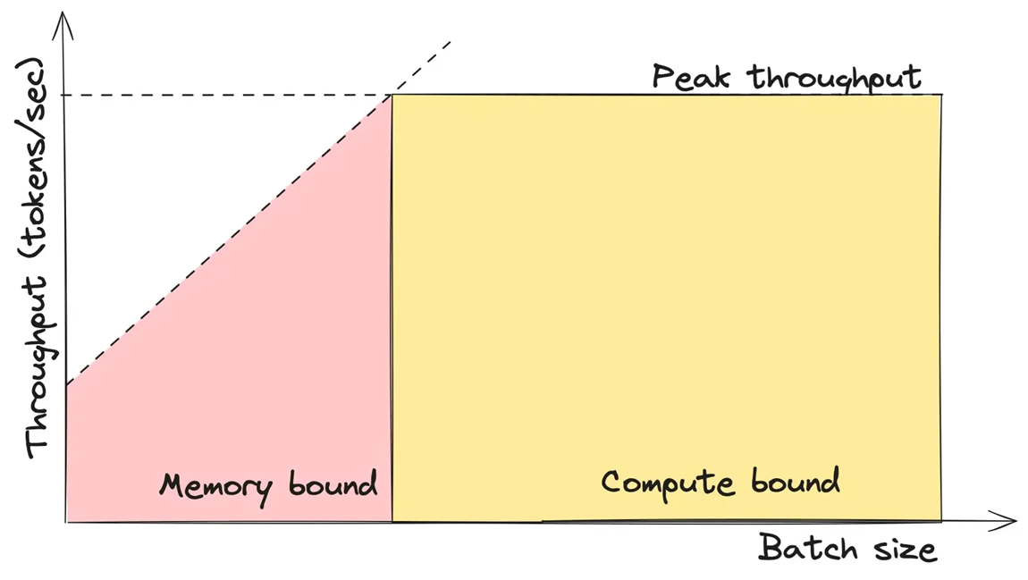
On this plane, there are two areas:
- When the batch size is small, the LLM operates in a memory-bound regime.
- As the batch size reaches a certain threshold, the model transitions to a compute-bound regime. We’ll discuss the intuition behind this a bit later.
Let’s use the factory metaphor again to get a rough understanding of this concept. Batch size is like the amount of raw materials delivered to the factory in a single shipment. The factory’s furnaces also have a maximum capacity for how much raw material can be processed at once. When the batch size is small, the factory can process the entire batch, so the throughput (the amount of raw material processed per unit of time) increases linearly. However, once the furnaces reach their peak capacity, the throughput can no longer increase; instead, any extra raw material will have to wait its turn. While this isn’t a perfectly accurate description, it helps illustrate the basic idea.
An important point here is that when the model is in the memory-bound area, its throughput increases almost linearly. However, in the compute-bound area, the throughput remains constant and reaches the peak throughput.
The peak throughput is the maximum throughput the model can achieve. It depends on several factors, including the model’s architecture, size, and the underlying hardware. Understanding how to calculate peak throughput involves analyzing the model’s computational demands and the capabilities of the hardware. We will explore this in detail shortly.
LLM inference math
In the previous section, we understood how to find batch size that optimally balances latency and throughput - it’s the size for which computation speed becomes equal to memory movement speed. Now, we’ll assess it for a particular LLM and a particular GPU model. And for that, we’ll need to get our hands dirty with math.
First, let’s examine what is typically stored in GPU memory during LLM inference:
-
LLM weights (parameters). This space is reserved for storing all the model parameters. The required memory size depends on the number of parameters and the floating-point precision used to store them. Parameters are often stored and used in FLOAT16 or BFLOAT16, unless quantized.
-
KV-cache. Stores keys and values for previous tokens to avoid recalculating them again an again. At the prompt processing stage, prompt tokens are processed in one forward pass, and the corresponding KV-cache entries are filled. At the autoregressive generation stage, cache is used for new computations and updated with keys and values of the last token, each time.
Cache size increases linearly with context length and with batch size. Its size also depends on floating-point precision.
-
Activations: This part of the memory is used to store intermediate data (neural network activations) during the current iteration of the LLM. The memory size required for activations depends on the framework implementation and the floating-point precision used.
Usually we assume it as constant and don’t consider in calculation
In the remaining part of this section we’ll make two takes towards computing the optimal batch size for a particular LLM and a particular GPU type:
-
For the first take, we’ll draft an approximate calculation ignoring KV-cache and LLM’s architectural details. We assume here that we work with relatively low context sizes, so that KV-cache size $\ll$ weights size.
-
For the second take, we’ll try to take into account transformer arhitecture, calculating flops for every operation and assuming the use of a KV-cache.
And the results will surprise us.
Take 1: a cache- and architecture-oblivious computation
Memory movement
Let’s estimate the amount of memory movement required to generate a single token. For a basic approximation, we assume that generating one token requires loading all of the LLM’s weights into the compute engine. (Again, we assume that KV-cache size $\ll$ weights size.) This means that the memory movement, $M$, can be estimated using the following formula:
\[M = N \cdot B\]where:
- N is the number of parameters of our LLM,
- B is the number of bytes used to store one parameter. For example, if the weights are stored in FP16 (16-bit floating-point) or BFLOAT16 (16-bit brain floating-point) - which is usually the case for LLMs - B would be 2 bytes, as each parameter requires $2 = 16\,\text{bits}/ 8\,\text{bits_per_byte}$ bytes of storage.
Note: For simplicity, we assume here that the context length is very short, so it can be ignored in future calculations.
FLOPs
To estimate the number of floating-point operations (FLOPs) required to generate a single token, we assume that each token needs to be multiplied by all the parameters, and then the results are summed across all parameters. While this is a rough approximation, it provides a useful starting point for calculations. The formula for estimating the number of FLOPs needed to generate one token is:
\[FLOP = 2 \cdot N \cdot batch\_size\]where N is the number of the LLM parameters.
Thus, for each parameter, we perform one multiplication and one addition. Since each operation counts as a floating-point operation, the total number of FLOPs is approximately twice the number of parameters for every token in the batch. You can find more details here.
Based on this, we can make a rough estimation of the LLM’s throughput. The formulas for calculating compute and memory movement times are:
\[\mathrm{time\_of\_computations} = \frac{\mathrm{FLOP}}{\mathrm{GPU\_peak\_FLOPs}}\] \[\mathrm{time\_of\_data\_movements} = \frac{M}{ \mathrm{GPU\_memory\_bandwidth}}\]The throughput
The throughput should be:
\[\mathrm{throughput} = \frac{\mathrm{batch\_size}}{(\mathrm{time\_of\_computations} + \mathrm{time\_of\_data\_movements}) }\]And we can also understand whether our inference is a memory bound or a compute-bound process:
\[\mathrm{Memory\ bound}: \mathrm{time\_of\_computations} \ll \mathrm{time\_of\_data\_movements}\] \[\mathrm{Compute\ bound}: \mathrm{time\_of\_computations} \gg \mathrm{time\_of\_data\_movements}\]These formulas give us an approximate yet powerful instrument to estimate the optimal batch size for our LLM.
Optimal batch size
Let’s return to the performance plane again.
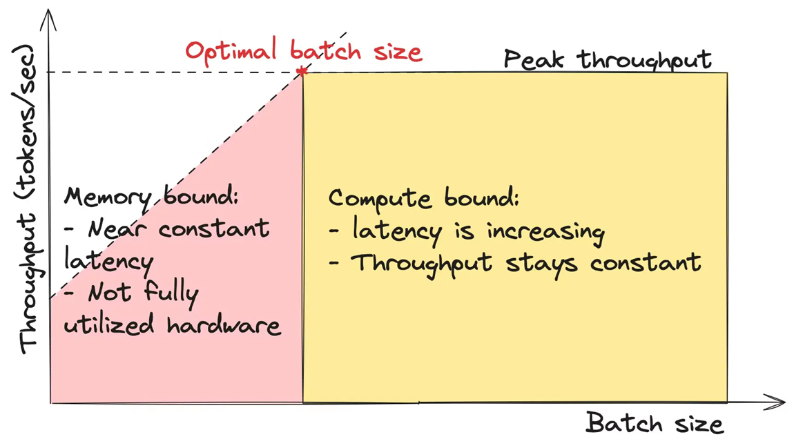
Now we can explore the characteristics of working in memory-bound and compute-bound regimes. When an LLM operates in a memory-bound regime, its latency remains relatively constant. This happens for two reasons:
- The time spent on data movement is significantly greater than the time spent on calculations.
- The time for data movement does not depend on batch size.
In this scenario, the hardware is not fully utilized because the calculations don’t take full advantage of the compute engines’ power. As a result, while latency remains stable, throughput increases linearly with batch size.
\[\mathbf{Memory\ bound}:\qquad \mathrm{time\_of\_computations} \ll \mathrm{time\_of\_data\_movements}\] \[\mathrm{throughput}_m(\mathrm{batch\_size}) = \frac{\mathrm{batch\_size}}{\mathrm{time\_of\_data\_movements}}\] \[\sim \frac{\mathrm{batch\_size}}{ \mathrm{Const}}\]In the compute-bound regime throughput stays constant but latency increases:
\[\mathbf{Compute\ bound}: \qquad \mathrm{time\_of\_computations} \gg \mathrm{time\_of\_data\_movements},\] \[\mathrm{throughput}_c(\mathrm{batch\_size}) = \frac{\mathrm{batch\_size}}{ \mathrm{time\_of\_computations}} =\] \[=\mathrm{batch\_size} \cdot \frac{\mathrm{GPU\_peak\_FLOPs}}{2 \cdot N \cdot \mathrm{batch\_size}} = \frac{\mathrm{GPU\_peak\_FLOPs}}{2 \cdot N}\]Thus, the optimal batch size is the point on a graph where we can achieve maximum throughput with minimal latency.
But first, let’s step back and return to our factory and warehouse analogy. Imagine we are producing steel (output tokens) as our product. The raw materials we need are coal (the model’s weights) and iron (input data). In this analogy, we need a constant amount of coal regardless of how much steel we produce, and the volume of coal is much larger than that of iron. So, the main challenge in the delivery process is getting the coal, while delivering the iron is almost negligible.
-
As we increase the batch size, the amount of coal stays the same, but we need more furnaces (CUDA cores) in our factory. Since many furnaces are idle, we don’t need additional time and can produce the steel in parallel. This means the system’s latency remains constant, while throughput—the volume of steel produced in the same time—increases. This is a memory-bound regime: the factory has many unused resources, making it underutilized.
-
At some point, as the batch size (or volume of iron) increases, we reach a point where all furnaces are in use, and we can no longer produce more steel in parallel. This means we must start producing goods sequentially. At this stage, the system’s latency begins to increase, but throughput remains the same. This is an example of operating in a compute-bound regime.
As you can see, the point at which all furnaces are in use is the point of optimal batch size.
In mathematical terms, the optimal batch size is the point where:
\[\mathrm{time\_of\_computations} = \mathrm{time\_of\_data\_movements}\]and it can be calculated as:
\[\mathrm{optimal\_batch\_size} = \frac{\mathrm{GPU\_peak\_FLOPS} \cdot B}{2 \cdot \mathrm{GPU\_memory\_bandwidth}}\]For H100 NVL GPU and float16, the optimal batch size is equal to 160:
\[\mathrm{optimal\_batch\_size} = \frac{1671\ \mathrm{TFLOPS}}{3.9\ TB/s} \approx 430\]An important note. You may be surprised that the optimal batch size doesn’t depend on the model size, and this requires some additional explanation. Our calculations takes into account two things: the speed of GPU computations and the speed of delivering data from GPU memory to the compute engine. This means, however, that both the data and the model weights are already stored in the GPU memory. So, our estimate is correct for infinite GPU memory. In practice, a batch of size 430 may be too large, and in this case,
$\text{true_optimal_batch_size} = \min(\text{optimal_batch_size; max_size_that_fits_into_the_GPU_memory})$
Even the LLM weights may be too large to fit into one GPU (imagine Llama 405B that would require at least 5 H100 GPUs to store weights only). For multi-GPU setup, the calculations become more tedious due to data channelling between GPUs.
Note. As previously mentioned, LLM memory consumption includes:
- Memory for weights: The space required to store all model parameters.
- Memory for cache: This depends on the batch size and context length and is used to store intermediate results.
For small models like Llama 8B, the practical batch size is often much lower than the theoretical limit (e.g., 430) due to the high memory consumption of activations and cache. As a result, LLM inference is predominantly memory-bound. To improve inference speed, focusing on optimizing memory movement is more effective than enhancing computational performance.
Take 2: Arhitecture-specific computation
Now, we’ll try to take into account transformer arhitecture, calculating flops for every operation and assuming the use of a KV-cache. However, as before, we’ll assume that LLM’s weights are already stored on a GPU. That’s logical for most practical setups; however, in some cases, when we’re low on GPU memory, we might offload parts of a model to CPU and drag them back and forth to GPU for computations - this, of course, makes everything more computationally expensive.
This time, we’ll need to take sequence length into account. Let’s denote by l_prompt and l_completion the lengths of prompt and completion respectively, and by seq_len the total prompt + completion length.
Let’s understand the inference cost of various LLM components.
A reminder about matrix multiplication cost
When we multiply two matrices
\[\underset{m\times n}{A} \cdot \underset{n\times k}{B},\]for each of the $mk$ elements of the product, we need to perform $n$ multiplications and $n-1$ addition, totaling to $2n-1\approx 2n$ FLOPs
\[(AB)_{ij} = \sum_ta_{it}b_{tj}\]In total, we get $\approx 2mnk$ FLOPs.
Self-Attention
Let’s go through the components. For the sake of simplicity, we’ll calculate flops per signle string of a batch, i.e. like we have batch_size = 1. We will add batch size to our calculations further down the road.
-
Query projection:
\[2\cdot\text{seq_len}\cdot\text{hid_dim}\cdot\text{num_heads}\cdot\text{head_dim}\text{ FLOPs}\](seq_len, hid_dim) x (hid_dim, num_heads * head_dim)gives us -
Key/Value projections:
\[2\cdot\text{seq_len}\cdot\text{hid_dim}\cdot\text{num_kv_heads}\cdot\text{head_dim FLOPs}\](seq_len, hid_dim) x (hid_dim, num_kv_heads * head_dim)give eachWe’ll have different number of query and key/value heads for grouped query attention.
Thanks to the KV-cache, each of these projections is performed only once for each token.
-
Output projection:
\[2\cdot\text{seq_len}\cdot\text{hid_dim}\cdot\text{num_heads}\cdot\text{head_dim}\text{ FLOPs}\](seq_len, num_heads * head_dim) x (num_heads * head_dim, hid_dim)also gives us -
Computing attention scores $S = QK^T$. This happens in different ways during the two attention stages:
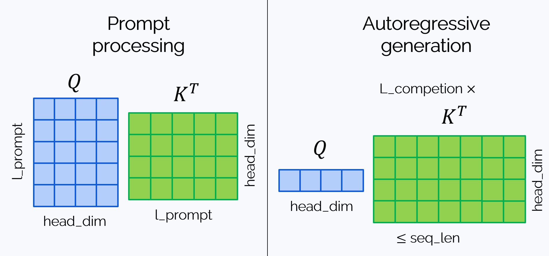
Over
\[2\cdot\text{l_prompt}\cdot\text{head_dim}\cdot\mathbf{l\_prompt}\cdot\text{num_heads}\leqslant\] \[\leqslant 2\cdot\text{l_prompt}\cdot\mathbf{seq\_len} \cdot\underbrace{\text{attn_hid_dim}}_{=\text{head_dim}\cdot\text{num_heads}}\text{ FLOPs}\quad{(P)}\]num_headsheads, the first stage requiresNote that we have
attn_hid_diminstead of justhid_dimhere. For most models, hidden dimensions inside attention layers is the same as hidden dimensions between transformer blocks, but there are some LLMs for whichattn_hid_dim != hid_dim. So, we distinguished between them here, just in case.As for the second stage, for each newly generated token we have, over
\[2\cdot\text{head_dim}\cdot\mathbf{\left(l\_prompt + l\_current\_completion\right)}\cdot\text{num_heads}=\] \[\leqslant2\cdot\text{head_dim}\cdot\mathbf{seq\_len}\cdot\text{num_heads}=\] \[=2\text{seq_len}\cdot\underbrace{\text{attn_hid_dim}}_{=\text{head_dim}\cdot\text{num_heads}}\text{ FLOPs}\]num_headsheads,We generate
l_completiontokens, which gives in total
Combining (P) and (C), we get the following upper estimate:
\[2\left(\underbrace{\text{l_completion} + \text{l_prompt}}_{=\text{seq_len}}\right)\cdot\text{seq_len}\cdot\underbrace{\text{attn_hid_dim}}_{=\text{head_dim}\cdot\text{num_heads}}=\] \[2\cdot\text{seq_len}^2\cdot\underbrace{\text{attn_hid_dim}}_{=\text{head_dim}\cdot\text{num_heads}}\text{ FLOPs}\]-
Computing attention output \(O=\text{Softmax}(M + S)\cdot V\). We can ignore softmax and masking and concentrate on multiplication of matrix of sizes not greater than
\[2\cdot\text{seq_len}\cdot\text{seq_len}\cdot\text{num_heads}\cdot\text{head_dim}=\] \[=2\cdot\text{seq_len}^2\cdot\text{num_heads}\cdot\text{head_dim}\text{ FLOPs}\](seq_len, seq_len) x (seq_len, head_dim), which happenshead_dimtimes:
The total computational cost is
\[C_{\text{attn}} = 4\cdot\text{seq_len}\cdot\text{hid_dim}\cdot\text{head_dim}\cdot(\text{num_heads} + \text{num_kv_heads}) +\] \[+ 4\text{seq_len}^2\cdot\text{head_dim}\cdot\text{num_heads}\]FFN
We’ll perform calculation for the most popular architecture to date, the gated MLP:
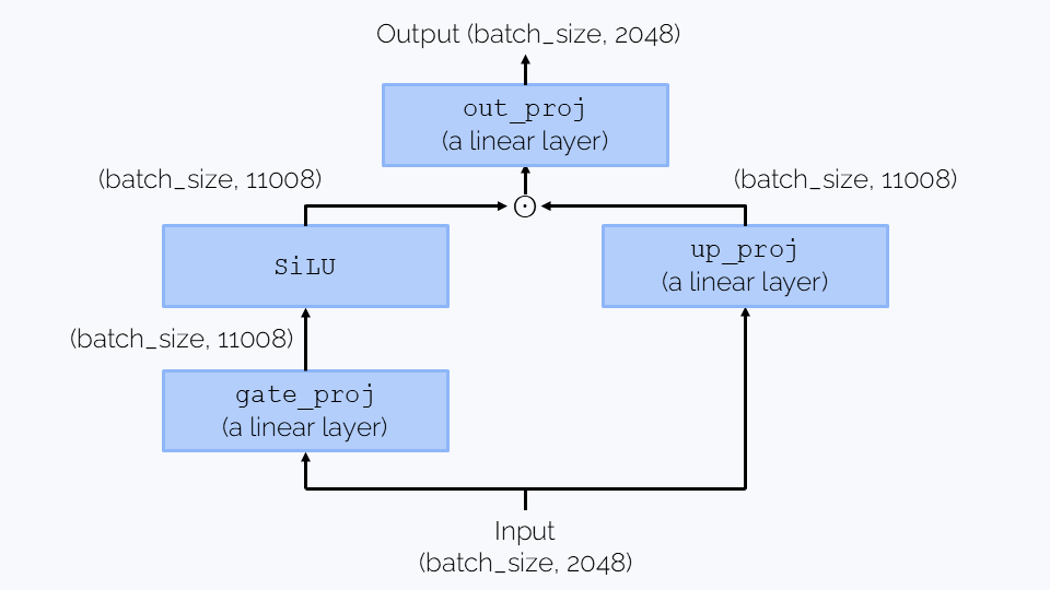
The computation is dominated by three matrix multiplications, each (seq_len, hid_size) x (hid_size, intermediate_size) or (hid_size, intermediate_size) x (seq_len, hid_size), which gives in total
Embedding and unembedding layers
Embedding layer is just a lookup table, so its computational cost is negligible. The unembedding layer performs matrix multiplication (seq_len, hid_dim) x (hid_dim, vocab_size), which gives
Getting all together
Now the total FLOPs can be computed as
\[C = \text{batch_size}\cdot(\text{n_layers}(C_{\text{attn}} + C_{\text{FFN}}) + C_{\text{unemb}})\]The memory can be estimated as
\[M = M_{\text{param}} + \text{batch_size}\cdot M_{\text{KV-cache}},\]where $M_{\text{KV-cache}}\leqslant\text{seq_len}\cdot\text{head_dim}\cdot\text{num_kv_heads}$.
Calculating for Llama-3.1-8B
Let’s recall the LLM’s parameters:
| Parameter | Value |
|---|---|
hidden_size |
4096 |
head_size |
128 |
intermediate_size |
14336 |
seq_len |
8192 |
num_heads |
32 |
num_kv_heads |
8 |
num_layers |
32 |
vocab_size |
128256 |
We took 8192 for seq_len - a deliberate choice, which is a good estimate for many day-to-day tasks. Then we have
Quite notably, at such context length attention computations don’t dominate the computation; but the situation will change as the sequence length will grow. Also, $C_{\text{unemb}}$ looks very large, but don’t forget that the other two numbers will get multiplied on n_layers.
Totally, we get
\[\text{FLOPs} = 19.3\cdot 10^9\cdot \text{batch_size}\]The memory size is
\[M = 16\cdot 10^9 + 10^9\cdot\text{batch_size}\]Optimal batch_size value for llama-3.1-8B
Let’s recall the formulas for computing computation and memory movement times:
\[\mathrm{computation\_time} = \frac{\mathrm{FLOPs}}{\mathrm{GPU\_peak\_FLOPs}} \\ \ \\\mathrm{data\_movement\_time} = \frac{M}{ \mathrm{GPU\_memory\_bandwidth}}\]Optimal batch size corresponds to the moment, when computation_time == data_movement_time:
From here, we find that the optimal batch_size equals $−16.75$.
What does this result mean? To understand it, let’s plot how FLOPs and data movement time behave as the batch size grows:
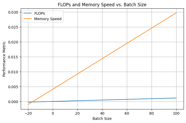
You can see that memory movement time grows faster than compute, so the LLM always stays in a memory bound regime. But don’t let it discourage you! There is a number of optimization techniques that help speed up the inference, and we’ll talk about some of them in Topic 5.