Paperwatch 28.05.2025 by Stanislav Fedotov (Nebius Academy)
New Models, Services, and Frameworks
Claude 4
https://www.anthropic.com/news/claude-4
The new family by Anthropic consists of two models: Sonnet and Opus. (The latter is somewhat surprising; I thought they stopped shipping Opus modes.) They are non-surprisingly good at coding and agentic tool usage.
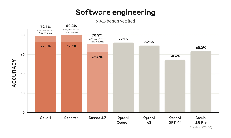

Like Claude 3.7 Sonnet, these models can work in straight-to-the point and long-reasoning regimes. Reportedly Opus is also good at working with memory – in particular, with creating and maintaining memory snapshots.
Anthropic also uncovered Claude Code, a coding agent that you can invoke from both terminal command line and several popular IDEs.
From my experiments, Claude 4 is less unruly in coding that Claude 3.7 that was prone to coming up with unasked for makeshift, panicked solutions. With Claude 4 I feel myself a bit more as working with a collaborator than having a talented but slightly crazy intern.
In creative writing, Claude 4 still suffers from the bane of all LLMs – contrived characters and formulaic plots with a general tendency to awkward symbolism and meaningless grandeur. However, in some cases it produces really nice, down-to-earth and relatable plotlines. So, maybe it will be my next favourite creative writing LLM after GPT-4o :)
VEO-3 by Google
https://deepmind.google/models/veo/ https://blog.google/technology/ai/google-flow-veo-ai-filmmaking-tool/
This is the video generation model (which also generates sound!) that makes you believe in custom movie endings The examples I’ve seen, however much cherry picked, are really crazy. Probably, soon we won’t be sure what’s real and what’s not… (I wish they had more about it in the Mission Impossible: Final Reckoning movie!)
OpenAI Codex
Several days earlier that Anthropic did, OpenAI announced their new
- Coding agent Codex that is now available for Pro+ (and hopefully will also be available for Plus…)
- An open-source coding agent Codex CLI :O that works from your terminal

I am a humble Plus user, so I can’t try it yet, but while exploring the docs, I noticed some features that might be good or not depending on your particular predicament:
- The Codex agent runs in a default container image, which comes pre-installed with common languages, packages, and tools – that’s as good a Colab, but if we move from a jupyter notebook to serious software engineering, having different experimenting/developing/production environments might punish you.
- OpenAI did some good steps towards establishing secure usage – for example, deleting secrets after initial setup.
Gemini Diffusion
https://blog.google/technology/google-deepmind/gemini-diffusion/
From time to time, researchers challenge transformer architecture in pursuit of something better – which usually means something faster. Once, State Space Models (including the famous Mamba) were a candidate transformer killers. Now, there are some experiments around Diffusion LLMs. Now, Google shipped such a model of their own. Alas, they only suggest joining the waitlist, so it’s not clear how much cool the new model is, but Google claims that it’s significantly faster than ordinary Gemini. If you’re curious and want to learn more about this new architecture, check the multimodal diffusion LLM review below.
Devstral
https://mistral.ai/news/devstral An open source coding LLM from Mistral and All Hands AI 🙌, which seems to outperform other open source coding LLMs, even (much) larger ones.
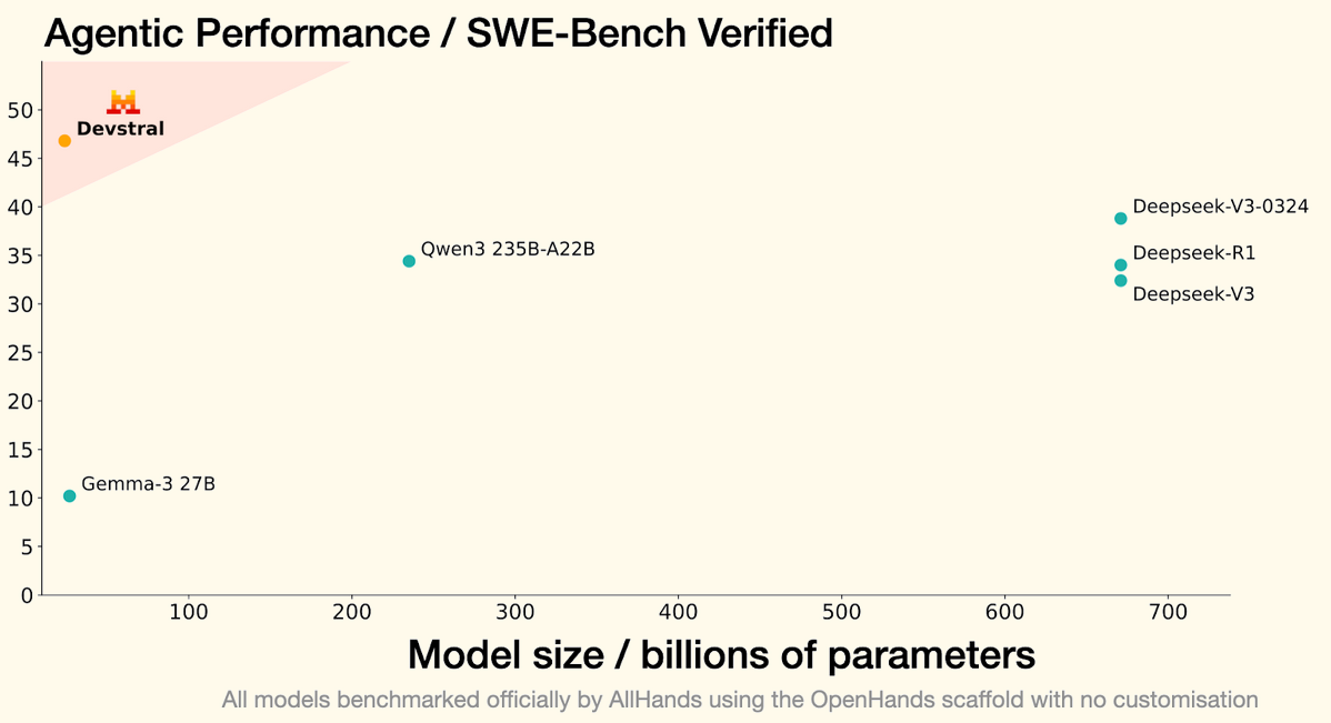
Devstral is trained to solve real GitHub issues; it runs over code agent scaffolds such as OpenHands or SWE-Agent, which define the interface between the model and the test cases.
With 24 billion parameters, Devstral is light enough to run on a single RTX 4090 or a Mac with 32GB RAM, making it an appropriate model for local deployment and on-device use :O
Do Language Models Use Their Depth Efficiently?
https://arxiv.org/pdf/2505.13898
The idea of interpreting how LLMs work internally is very captivating, and once in a while, interesting papers appear revolving around mechanistic interpretability. Here’s one of them, and it analyses what transformer layers do. This question has a long and interesting history; some relevant research including
-
Transformer layers as painters, introducing the idea of middle layers having some subtle specializations, like a painter receiving the canvas from the painter below and deciding whether to add a few strokes to the painting or just pass it along to the painter above her (using the residual connections).
A very interesting observation made by the authors was that in many cases (with notable exclusion of reasoning-heavy tasks) middle layers might be omitted or reordered without catastrophical quality degradation.
-
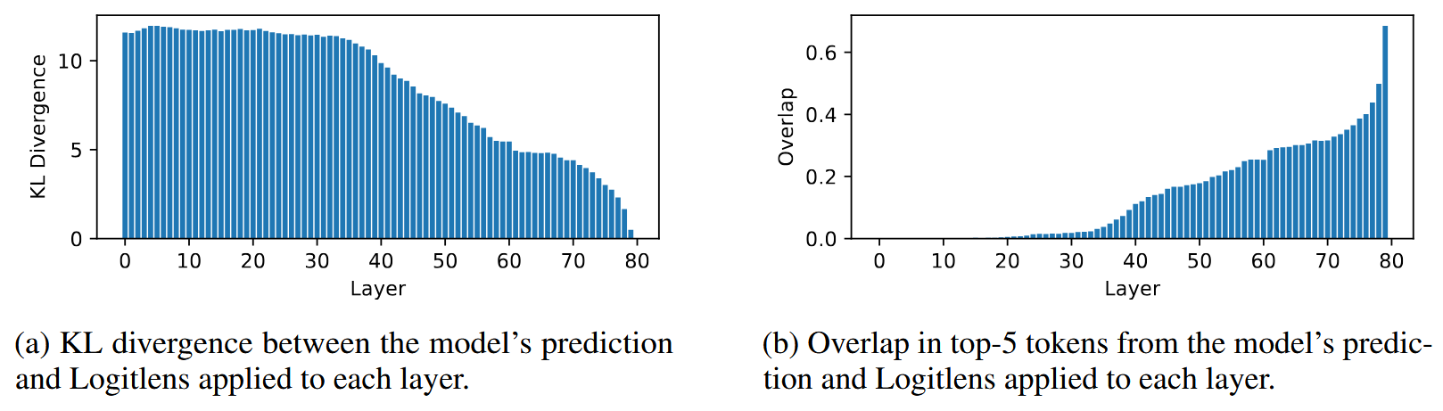
Logit lens, which is a nice tool for peeking into the transformer internals. How it works: after each transformer layer, we may apply the unembedding layer and look at the predicted tokens. Curious ways in which these predictions change from the bottom to the top layers might sometimes bring curious insights.
This paper also hints that some layers are slacking, but it gives this another perspective. A transformer layer has two main components – self-attention and FFN (with additional normalization here and there), and each of them is added alongside a residual connection, like, having the initial hidden state $h_{l}$:
\[\hat{h}_{l} =h_{l}+ SelfAttention\left(Norm\left(h_l\right)\right)\] \[h_{l+1}=\hat{h}_{l}+MLP(Norm\left(\hat{h}_{l}\right))\]This might indeed allow a transformer block not to do contribute much and to just leave $h_{l}$ mostly as it was. And a natural way of checking this is comparing magnitudes of the initial $h_{l}$ and of the things being added to it (“layer contributions”) while producing $h_{l+1}$:
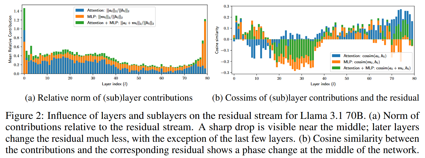
The authors observe (left plot above) that middle layers contribute significantly less than the first and several last layers.
The second plot is quite peculiar. The authors measured cosine similarity between $h_{l}$ and the sublayer contributions – and it seems to follow a distinct patterns, which the authors interpret in the following way:
- The first half of the layers tend to erase the residual, refining the features.
- In the second half, the model starts strengthening existing features instead of erasing information. This is not the only curious thing about the second half of the model! In the next experiment, the authors perform invasive testing. Taking some $t$, they run a transformer in two modes:
- Without intervention, obtaining downstream representations $h_{s}$ ($s>t)$
- Switching off the layer $f_{t}$ in $h_{t+1}=h_{t}+f_{t}$ and obtaining modified $\overline{h}_{s}$
Then they compute the relative contribution of $f_{t}$:
\[\frac{\|\left(h_{s+1}-h_{s}\right)-\left( \overline{h}_{s+1} - \overline{h}_{s}\right)\|_{2}}{\|h_{s+1}-h_{s}\|_{2}}\]The left plot below shows these numbers, max’ed over a sequence across a number of prompts, and you can see that the second half of the layers contributes significantly less!
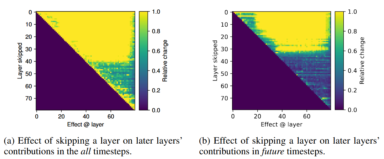
The authors conclude that the second half of the model refines the output probability distribution based on the information already present in the residual.
Another interesting experiment (the right plot on the picture above) shows effect of layer skipping for prediction of future tokens (not the current one). That is, layers are only skipped over tokens before the one that is generated at the moment.
Here, the picture is even more impressive, validating the hypothesis: that the second half of the network is merely doing incremental updates to the residual to refine the predicted distribution. A similar effect surfaces in the analysis of Logit Lens outputs: it’s in the second half of the network that these outputs start resembling the actual LLM predictions.
Transformer depth vs long computations
Inference-time compute is a big thing now, and understanding how exactly LLMs perform long reasoning is an important thing in mechanistic interpretability. A reasonable hypothesis might be that for problems requiring long solutions, more layers will be used – because there is no horizontal information exchange inside a transformer layer (in contrast to RNN), and we only have as many chances to perform information exchange across the sequence as we have self-attention layers.

However, in their experiments the authors see no proofs of increasing involvement of second-half layers with growing complexity of a problem – like taking a multi-hop task. (It might be that they just didn’t increase the complexity enough…) Also, no novel computation patterns seem to arise with increasing model depth. (But again, it might be that the authors didn’t try problems complicated enough – who knows.)
Interestingly though, a Universal Transformer model trained by the authors exhibit increasing “useful depth” with increasing problem complexity. It would be interesting to see further developments in this topic.
Beyond Semantics: The Unreasonable Effectiveness Of Reasonless Intermediate Tokens
https://arxiv.org/pdf/2505.13775
This is another paper reinforcing the opinion that tokens produced by a long-reasoning model during the reasoning phase shouldn’t necessary be thoughts.
As a number of papers before it, this one analyses long reasoning through the perspective of pathfinding – approximation of A* algorithm with LLMs. It is indeed a tempting path: a pathfinding algorithm produces
- a trace describing all attempts at finding the right path – this is a direct analogy of a non-linear reasoning and
- a plan which is a final solution.
An LLM may be trained from scratch on these traces and plans thus learning to cope with mazes. The authors generate a number of mazes with Wilson’s Algorithm (see, for example, this post for an explanation and some visualizations, or check the paper itself), run A* in them and train an LLM in three ways:
- On plans (solutions) only
- On plans and traces (solutions + long reasoning)
- And now, the most interesting one: on plans and traces from different mazes. Which means, a trace is totally irrelevant to a plan apart from the fact that they come from the same maze universe.
Now, you’d bet that the third way won’t produce anything working, and you’d be wrong!
The authors tested their LLMs on mazes generated by several different algorithms, not only Wilson’s.
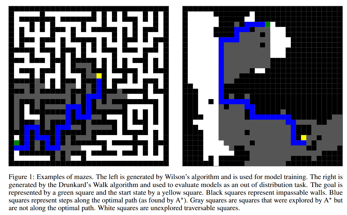
One of these algorithms is the Drunkard’s Walk which produces cave-like systems that are severely out-of-distribution for an LLM trained on neat Wilson’s mazes.
Now, here are the results:

The authors checked both Trace and Plan validity, and they observed a very curious thing: the LLM trained on swapped trace-plan pairs, despite producing incorrect traces, performs better than the conventionally trained model and even generalizes better to OOD Drunkard’s Walks!
Now, isn’t this another hint that true reasoning happens deep inside an LLM and might be not connected directly to the “though-like” outputs? (Another similarly powerful hint is Let’s Think Dot By Dot, of course.)
When Thinking Fails: The Pitfalls of Reasoning for Instruction-Following in LLMs
https://arxiv.org/pdf/2505.11423
LLM Reasoning is often beneficial, but sometimes not. For example, the To CoT or not to CoT paper established that Chain-of-Thought reasoning doesn’t help (and sometimes can even hurt) in knowledge-related questions. Now, what about long reasoning? Can it hurt? The authors of this paper investigate several situations where it indeed can make things worse. Namely, they discuss the issues of LLMs getting carried away and/or adding some well-intentioned though redundant information in the response – and this violating simple constraints such as word count limits, answer formatting etc.
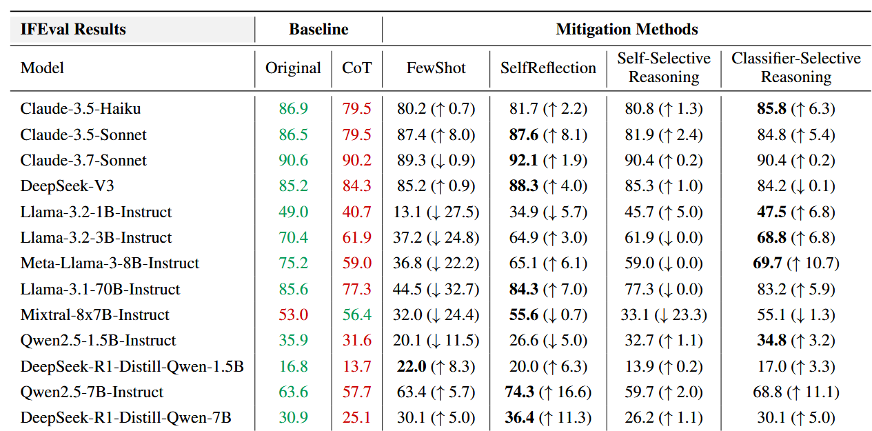
In my opinion, it’s a bit strange to expect from a long reasoner to abide to such down-to-earth constraints; they are needed for different scenarios – and if one needs an answer in $\leqslant 100$ words or an answer in a very specific format, that can be established with post-processing. It’s not surprising that in the end the authors observe that the best way of countering this problem is Classifier-Selective Reasoning – using a classifier (another LLM) to decide whether long reasoning is needed, before actually asking the main LLM to produce the solution.
I very much agree with such a setup. Despite universal love towards long reasoning, it’s often redundant. So, it’s important to distinguish in which cases to use it and in which cases to refrain from it.
A table with motivational numbers:
Parallel Scaling Law for Language Models
https://arxiv.org/pdf/2505.10475
If you worked with Classical ML, you probably remember an ensemble technique called Bagging. Bagging suggest taking several powerful models and aggregating their predictions to get the final result. But not just any models – they should be sufficiently different. For example, in Random Forest they took trees trained on different data subsets and with different feature subsets. An echo of this is the familiar Self Consistency – aggregating results of several LLM runs under non-low temperature, where thank to the stochasticity of generation, each run produces different results.
And no, I’m not just overcome with nostalgia; all of this is relevant to the Parallel Scaling Law paper The authors ponder the ways of scaling LLM power, criticizing the familiar Parameter Scaling and Inference Time Scaling (say hi to long reasoning and the almost forgotten now Tree of Thoughts) and suggesting a new paradigm – Parallel Scaling.

Parallel Scaling, as they describe it, resembles both Bagging and Boosting at the same time. The idea is, having a single base model $f_{\theta}$ and an input $x$:
- Apply $P$ learnt transformations to $x$, transforming it into $x_{1},x_{2},\ldots,x_{P}$
- Run $x_{1},x_{2},\ldots,x_{P}$ in parallel through the model $f_{\theta}$ (parallel execution here makes things more efficient in comparison with sequential long reasoning)
- Aggregate the results with some learnable function, for example,
with learnable $w_{1},\ldots w_{P}$.
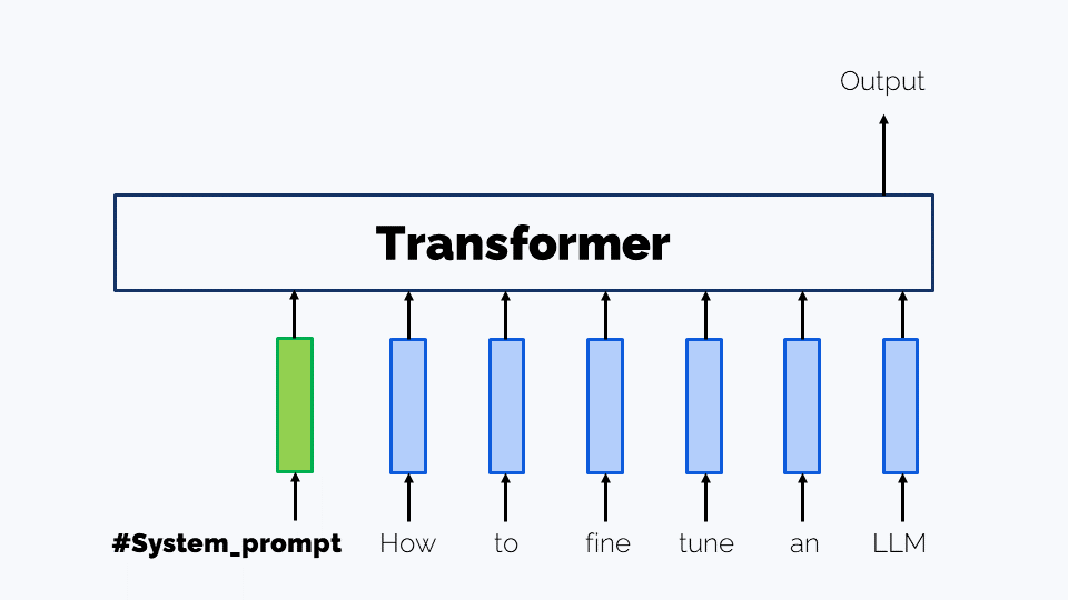
As the initial transformation of $x$, the authors suggest Prompt Tuning: prepending the prompt with learnable embeddings of “virtual tokens”.
But that’s not all! The authors decide to find a scaling law for this new configuration, connecting
- The number of model parameters $N$
- The achievable loss $L$
- The number of parallel streams $P$ – and, along with it, a number characterizing the diversity of these streams – as we remember well, it’s really important.
They start with the well-known Chinchilla Scaling Law, “forget” about the dataset-size-related summand and mathematically infer the law for the parallel stream configuration:
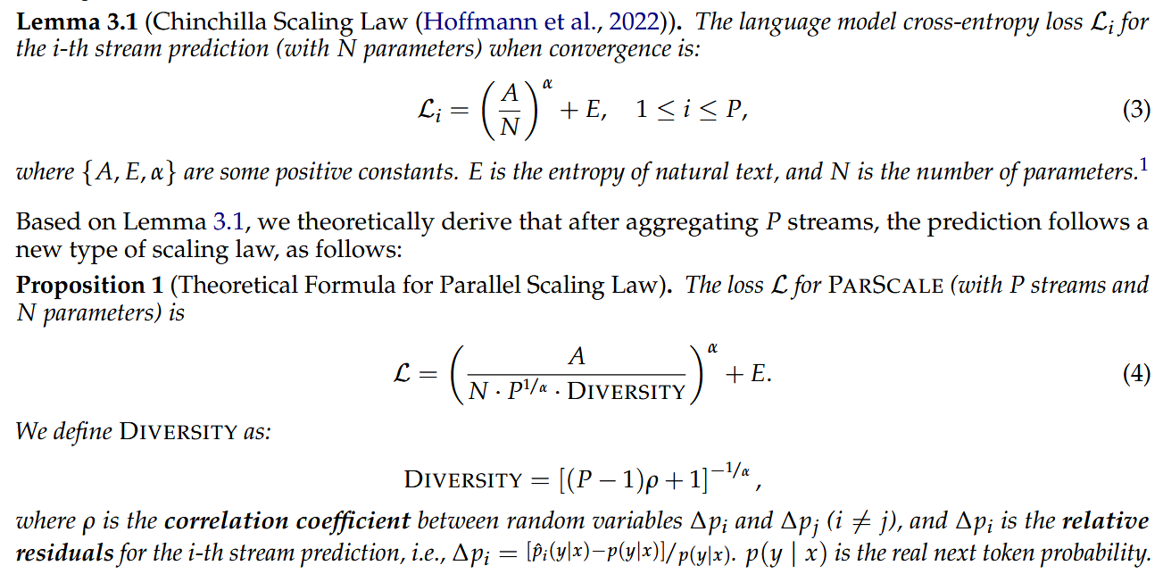
Then they fit the parameters $A$, $\alpha$ and $E$ with a proxy $k \log{P} + 1$ for the diversity.

What they observe is that with parallel scaling, they are able to get better loss with less memory and latency increase.
It’s important to note, however, that they train their models on a relatively small dataset of 42 billion tokens (trillion-size datasets are common in LLM training), which might influence the observations, because actual scaling laws also contain data-dependent terms. To address this, the authors also:
- train a 1.8B model (with 1.6B non-embedding parameters) on 1T tokens. In this scenario, they use two-stage training to avoid spending $P$ times more compute on each and every token:
- On 98% of the data the model is trained in an ordinary way
- And only then it’s trained in the parallel setup, on the rest of 2% data.
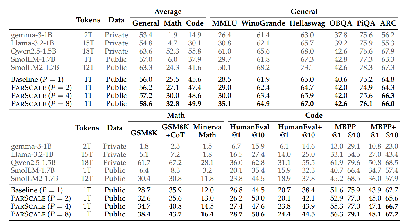
- apply their technique to Qwen-2.5 under two settings: continual pre-training and parameter-efficient fine-tuning (PEFT).
The results are quite promising:
Avoid Recommending Out-of-Domain Items: Constrained Generative Recommendation with LLMs
https://arxiv.org/pdf/2505.03336
LLMs are a promising tool for recommender systems: indeed, treating the customer’s previous actions as previous tokens, LLMs might predict potential recommendations as well as they predict next tokens. Of course, it’s useful to ensure output structure to be able to parse recommendations; for example, we might force the LLM to output
1. <SOI> \{\{recommendation 1\}\} <EOI> 2. <SOI> \{\{recommendation 2\}\} <EOI> ...
with special tokens <SOI> and <EOI> to mark the beginning and the end of the recommended titles.
A problem is, however, that we don’t want an LLM to be overly creative in the process – i.e. we’d like to avoid hallucinations and ensure that an LLM only predicts actual goods. This paper considers two ways of doing it.
-
The first approach (RecLM-ret) combines LLMs with retrieval in a creative way
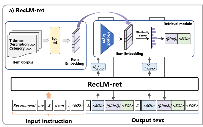
The authors suggest, as we encounter the
<SOI>token:- take the final embedding that the LLM produces from it
- project this embedding into the space of goods’ embeddings with a trainable MPL
- for the resulting vector, find the closest goods’ embeddings, and based on this, return the recommendation
- finally, the recommendation is inserted into the LLM’s generation stream as
- and after that, the LLM is again allowed to generate freely.
-
The second approach, RecLM-cgen, uses a prefix tree-constrained generation strategy
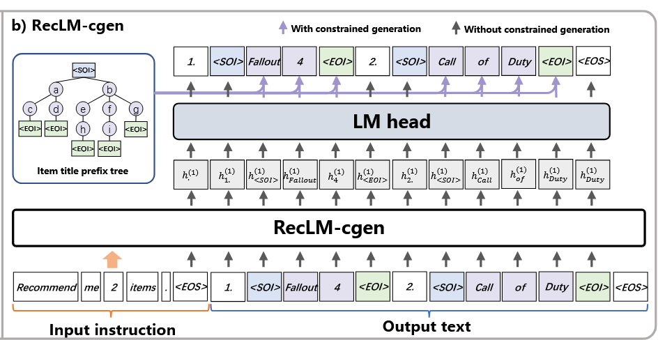
From the moment
<SOI>is generated, this strategy makes an LLM generate not just any tokens but the ones from a prefix tree of all items, according to their predicted probabilities. For example, if our items are “Fallout 2, Fallout 3, Falldown, Call of Duty, Call of Cthulhu”, the prefix tree might be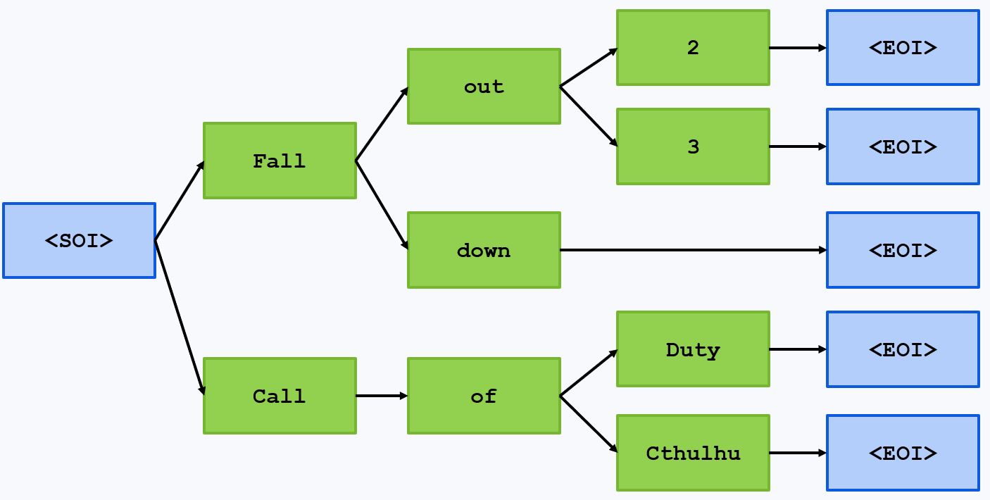
Then, after
<SOI>, the LLM will only be able to choose between Fall and Call; if these tokens get probabilities 0.1 and 0.2, they will be renormalized as $\frac{0.1}{0.1+0.2}=\frac{1}{3}$ and $\frac{0.2}{0.1+0.2}=\frac{2}{3}$, and either Fall or Call will be sampled according to these new probabilities. Then, if Fall is chosen, one of the tokens $out$ and $down$ will be predicted based on the probabilities predicted by the LLM from “...<SOI> Fall”When
<EOI>is finally reached, the LLM is again allowed to generate whatever it wants – until the next<SOI>.
Of course, you need to train (or at least to fine tune) and LLM to generate things this way. The authors collect a dataset from real users’ choices and recommendations by a powerful non-LLM recommender. With some additional loss function tricks, they train the LLM and get quite good results.
Overall, it’s a good study of how to tackle with hallucinations in specific production situations.
MMaDA-8B: Multimodal Large Diffusion Language Models
https://arxiv.org/pdf/2505.15809
The authors of this paper seek a way of creating models capable of native cross-modality generation and reasoning.
We’re already not hopeless in this. Early fusion Multimodal LLMs such as – I suppose – the today’s version of GPT-4o, are already capable of interleaving text and images. It must be the thing powering GPT’s image editing capabilities – as well as the mechanism that allowed GPT-4o to generate the cat on the right to the prompt “Generate an art showing the most popular kind of animal among the people of Istanbul.”.

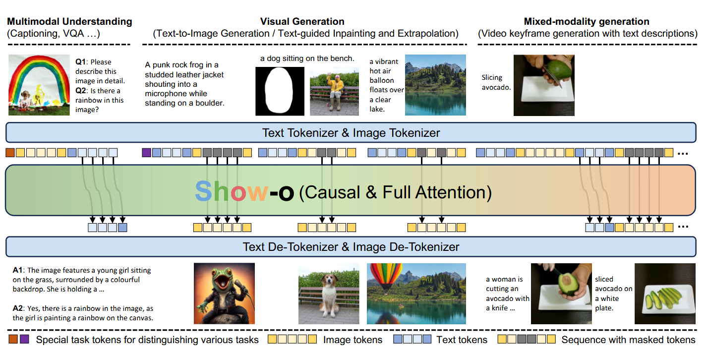
Early-fusion models, like show-o on the image below, establish native multimodality by creating a joint pipeline for image and texts tokenization and de-tokenization. For text, nothing changes in comparison with ordinary LLMs, while for images, an encoder (smth like VAE or VQ-VAE) is used for tokenization and latent diffusion + (VQ-)VAE-like decoder serve as de-tokenizer. And all of this might be trained end-to-end:
However, show-o and other open source Multimodal LLMs aren’t perfect yet, and the authors of this paper failed to create an Istambul’s cat using them. So, they try Diffusion LLMs as an architectural alternative. Diffusion LLMs iterate on the idea of Diffusion: there is a forward (noising) process and a backward process to reconstruct an object from noise.
In the original Diffusion LLM paper, this was done with masking/mask prediction:

The training had two stages:
- On the pre-training stage, the LLM was trained to predict masked tokens from any position
- On the instruction tuning stage, the LLM was trained to do the following: starting from a completely masked answer, it was trained to unmask it, token by token or token group by token group). Now, how to make this multimodal?

The architecture has a transformer at its core, working with text and vision tokens. An important thing to note here is that image encoders and decoders in MMaDA work with discretized image representaions – i.e., any image is described by a sequence of discrete tokens from a finite vocabulary. This allows to build a uniform pipeline for processing image and text alike in the same way as in the Diffusion LLM paper, with even a pre-training loss that is uniform across modalities.
Now, while pre-training is largely the same as for Diffusion LLMs, the interesting part starts when it comes to establishing long-reasoning capabilities. It is a two-stage process:
- Cold-start CoT fine tuning on a compact but good quality dataset of textual reasoning, multimodal reasoning, and text-to-image generation – the examples are obtained from the existing multimodal LLMs.
-
Unified GRPO
Well, no long reasoning paper without RL, isn’t it?
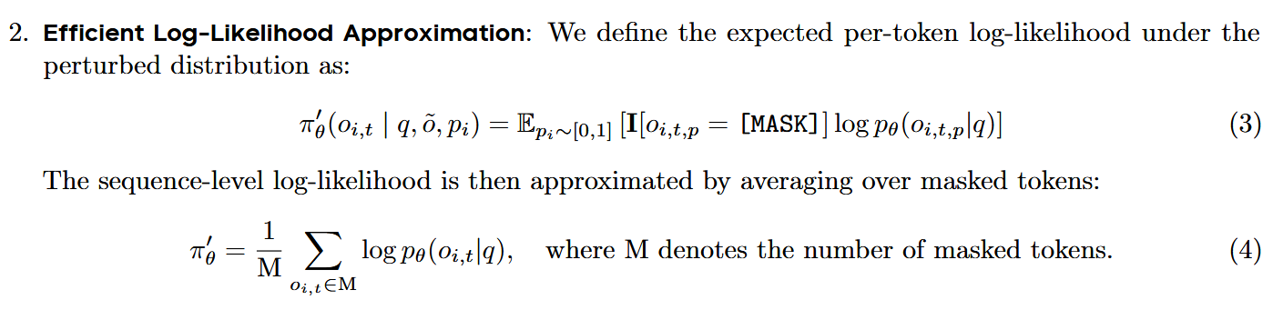
The main challenge here was to adapt GRPO to non-autoregressive setup – it’s not clear what to do with masked tokens. Policy values for them are estimated like this:
Apart from this, it’s more or less the same old GRPO:

with the loss
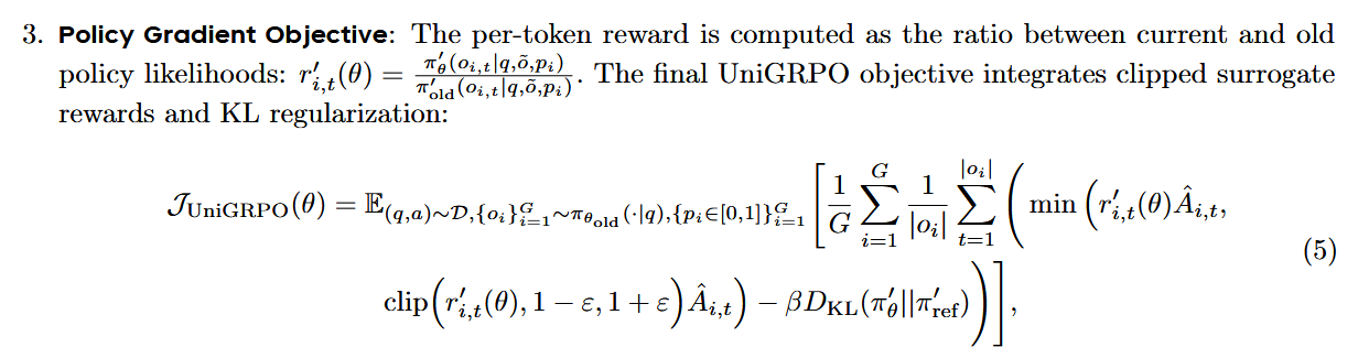
where the advantage has the usual form
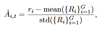
An interesting question, however, is how to define rewards. In text-only long-reasoner training, it’s format + answer (usually for math problems), but in multimodal settings it becomes more diverse. Here’s what the authors choose:
- Textual Reasoning Rewards: the usual answer correctness + checking the
<think>...</think>format abiding. - Multimodal Reasoning Rewards: For math-related (geometry) tasks such as GeoQA and CLEVR, it’s the same correctness and format. In addition, for caption-based tasks, CLIP Reward is used: $0.1 \cdot CLIP(image, text)$.
- Text-to-Image Generation Rewards: For image generation tasks, the same CLIP Reward is used + an Image Reward that reflects human preference scores. Both rewards are scaled by a factor of 0.1 to ensure balanced contribution during optimization.
- Textual Reasoning Rewards: the usual answer correctness + checking the
Here is what the results look like:

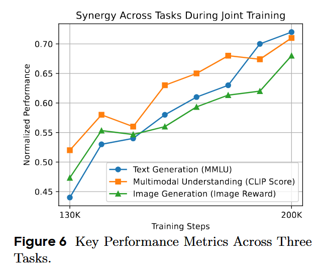
A curious thing observed during training is synergy across different modalities:
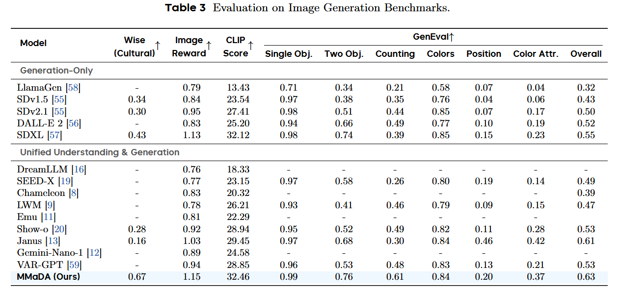
Here’s the numerical evaluation. No Qwen 3 on board, unfortunately, and not even recent Llamas :/
J1: Incentivizing Thinking in LLM-as-a-Judge via Reinforcement Learning
https://arxiv.org/pdf/2505.10320
As much as we love benchmarking LLMs on datasets where clear, easily comparable answers are available, in real life we often need to evaluate things like helpfulness, or toxicity, or retrieved context relevance, and there might be just no workaround to avoid using LLM-as-a-Judge.
But how to make an LLM as expert judge? By throwing in some inference-time compute – for example, by teaching the LLM to reason. And when we need long reasoning, RL comes to play. The authors explore training for either of the following working modes:
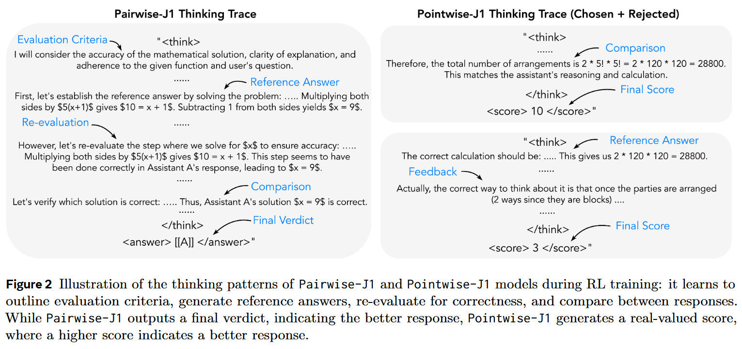
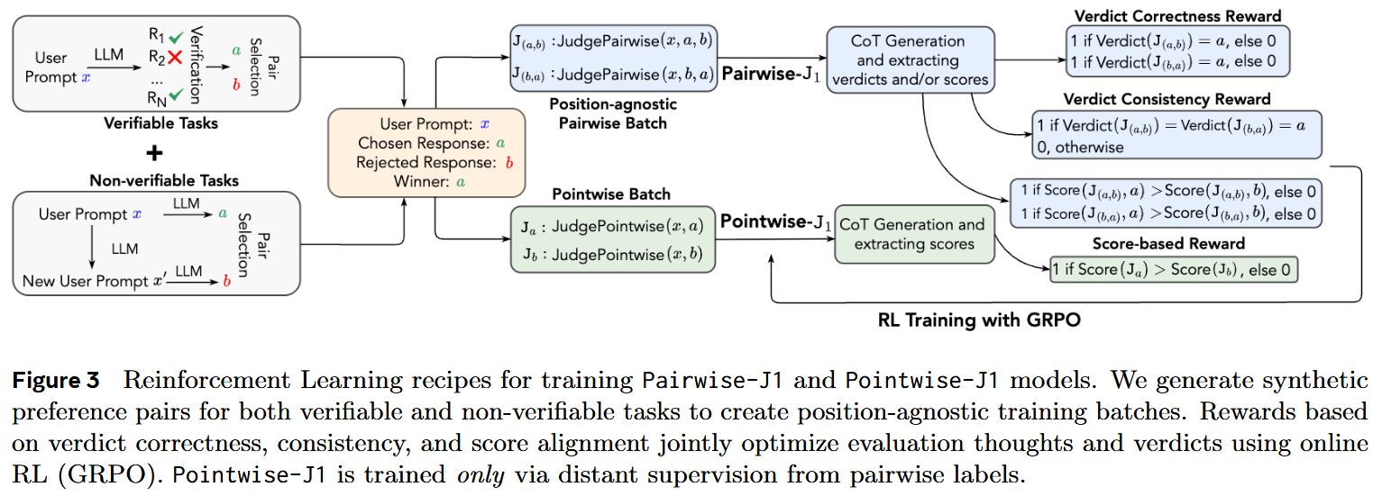
- Pairwise-J1 receives a user question and a response pair, and generates thought tokens and the preferred response (as the final verdict). (The authors also consider a version that output scores)
- Pointwise-J1 takes an instruction x and a single response a as input, and outputs a score (0 to 10) that reflects the quality or reward of the response.
Evaluation data As always, an interesting question is where to get data for evaluation of a trained Judge. That’s what the authors use (it was interesting for me to browse through available datasets):
- Preference Proxy Evaluations (PPE) – a large-scale benchmark that links reward models to real-world human preference performance. It consists of two subsets:
- PPE Preference (10.2K samples) - human preference pairs from Chatbot Arena featuring 20 LLMs in 121+ languages,
- PPE Correctness (12.7K samples) - response pairs from four models across popular verifiable benchmarks (MMLU-Pro, MATH, GPQA, MBPP-Plus, IFEval).
- JudgeBench (350 preference pairs; subset with responses generated by GPT-4o) - challenging response pairs that span knowledge, reasoning, math, and coding categories; the comparison in these pairs was made with priority for factual and logical correctness as opposed to stylistic alignment etc.
- RM-Bench (4K samples) a dataset that assesses the robustness of reward models based on their sensitivity and resistance to subtle content differences and style biases.
- FollowBenchEval (205 preference pairs) tests reward models for their ability to validate multi-level constraints in LLM responses (e.g., “Write a one sentence summary (less than 15 words) for the following dialogue. The summary must contain the word ‘stuff’…”).
- RewardBench (3K samples), similar to JudgeBench, consists of preference pairs from 4 categories of prompts: chat, chat-hard, safety, and reasoning.
Training data
For training, the authors use synthetic data, with prompts from 17K WildChat and 5K MATH and pairs of accepted/rejected answers obtained as follows:
- For WildChat, by prompting an LLM with an original prompt and with a “noisy” variant of it
- For MATH, by sampling several solutions and choosing as accepted a one with a correct answer and as a rejected – a one with an incorrect answer. The authors made efforts to counter position bias – a phenomenon, wherein the verdict changes if the order of the responses is swapped. To mitigate it, they always put both orders of response pairs – (x, a, b) and (x, b, a) – in one batch.
Training of Pairwise-J1 The Judge LLM is trained with RL, with the following reward models:
- Verdict Correctness Reward.
- Verdict Consistency Reward. In particular, the authors only assign a reward of 1 when the model produces correct judgments for both input orders of the same response pair (i.e., (x, a, b) and (x, b, a)).
- Format reward
Training of Pointwise-J1 This a tricky task, because the authors had no ground truth 0-10 labels. So this model was actually trained by distant supervision from a pairwise model in the following way: given a triplet (x, a, b) of a prompt x, an accepted answer a and a rejected answer b, the Pointwise LLM-as-a-Judge is trained to assign a score between 0 and 10 to a given response – in such a way that score(a) > score(b). This very much resembles how pairwise ranking models work, but with LLMs.
Results
The authors train Judge models of two sizes, and they turn out to be quite good.
