Introduction

While Supervised Fine Tuning trains LLMs on pairs $(query, answer)$, explicitly showing to an LLM what to generate, in some cases it may be too difficult (or even impossible) to create such a training dataset. In these cases, Reinforcement Learning (RL) might save the day. Let’s look at several particular situations.

1. Establishing LLM alignment with human preferences and values, making an LLM harmless and helpful. This may include it being non-toxic, resistant to jailbreaks, a good conversationalist etc.

It may be complicated to train an LLM for all that by showing only positive examples. A better idea would be to give the LLM both positive and negative signal by rewarding it for generating aligned completions and punishing for misaligned generation. This way, it might learn the boundary between good and evil.

This type of RL training requires a reward model - a special neural network that scores each completion, predicting its reward (which might be positive or negative). It is trained on pairs (prompt + accepted completion, prompt + rejected completion). Though it’s additional work, training a reward model that distinguishes alignment from misalignment, is much easier than generating a high-quality, large, and representative set of aligned (prompt, completion) pairs.

1. Training long reasoners such as DeepSeek-R1 or Qwen3. Though SFT may also be used to train an LLM to generate long, non-linear reasoning, gathering a high-quality dataset of non-linear solutions for such training is tedious. On the other hand, with RL, you only need the problems and the answers - no solutions at all! It turns out that a well-pre-trained model will emerge as a long reasoner with as little training signal as:

• Answer supervision - reward for the correct answer

• Format supervision - reward if the model abides an html format such as <think>...</think> <answer>...</answer>

During training, LLM generates solutions to given problems - and the feedback described above helps the training algorithm to steer an LLM towards giving correct answers and, quite unexpectedly, towards generating long, non-linear solutions.

1. Fine tuning LLMs to perform agentic tasks in complex environments. Examples might include

• Multi-turn web information retrieval, see WebDancer

• LLM-orchestrated application interaction scenarios, such as web shopping (“Return my last ordered Amazon t-shirt and buy it one size larger”), see AppWorld for examples of tasks and Reinforcement Learning for Long-Horizon Interactive LLM Agents for an example of an agent

• And even playing games, see RAGEN

In such scenarios, SFT isn’t feasible. Even if we could gather a large dataset of “correct” action sequences, it’s very important for the agent to make mistakes and learn on them. With that, RL helps.

Reinforcement learning in a nutshell

You may skip this section if you have already read it in the LLM Training Overview long read.

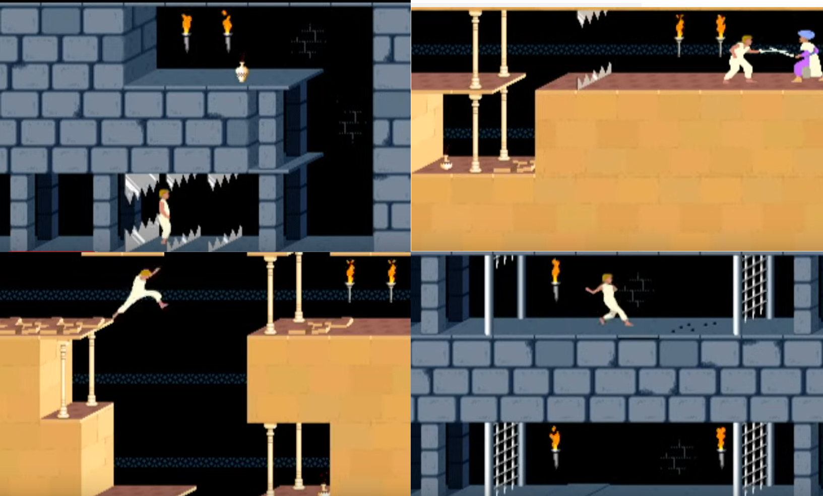
Imagine you want to train an AI bot to play Prince of Persia (the 1989 game). In this game, the player character (that is, the titular prince) can:

• Walk left or right, jump and fight guards with his sword
• Fall into pits, get impaled on spikes, or killed by guards
• Run out of time and lose
• Save the princess and win

The simplest AI bot would be a neural network that takes the current screen (or maybe several recent screens) as an input and predicts the next action – but how to train it?

A supervised learning paradigm would probably require us to play many successful games, record all the screens, and train the model to predict the actions we chose. But there are several problems with this approach, including the following:

• The game is quite long, so it’d simply be too tiresome to collect a satisfactory number of rounds.
• It’s not sufficient to show the right ways of playing; the bot should also learn the moves to avoid.
• The game provides a huge number of possible actions on many different screens. It’s reasonable to expect that successful games played by experienced gamers won’t produce data with the level of necessary diversity for the bot to “understand” the entire distribution of actions.

So, these considerations have us move to consider training the bot by trial-and-error:

1. Initializing its behavior (“policy”) somehow.
2. Allowing it to play according to this policy, checking various moves (including very awkward ones) and to enjoy falling to the bottom of a pit, and so on.
3. Correct the policy based on its success or failures.
4. Repeat step 2 and 3 until we’re tired of waiting or the bot learns to play Prince of Persia like a pro.

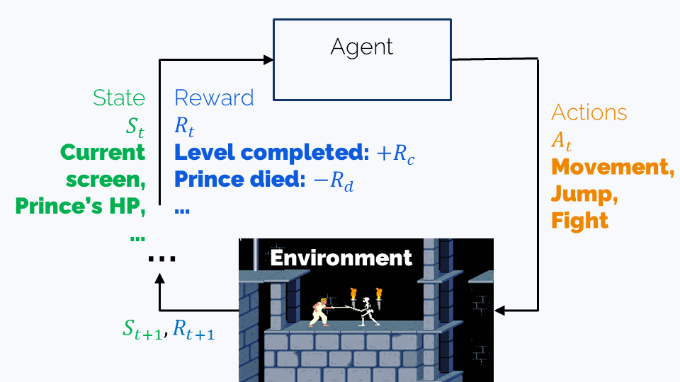
Let’s formalize this a bit using conventional RL terminology:

• The (observed) state is the information we have about the game at the present moment. In our case, this is the content of the current screen.
• The agent is a bot which is capable of several actions.
• The environment is the game. It defines the possible states, the possible actions, and the effects of each action on the current state – and which state will be the next.
• The policy is the (trainable) strategy the bot uses for playing. In our case, this is the neural network that predicts actions given the current state, or the state history.
• The reward is the score that we assign to an action performed in a certain state. For example, defeating a guard, progressing to a next level, or winning the game might have positive rewards, while falling into a pit or getting wounded by a guard would mean negative rewards.
• A trajectory is a particular sequence of states the agent finds itself in and actions it takes. In the Prince of Persia example, the whole playthrough will be a trajectory.

The goal of the training is finding a policy that maximizes reward, and there are many ways of achieving this. We’ll now see that alignment training has much relevance with Prince of Persia.

Reinforcement Learning for LLMs

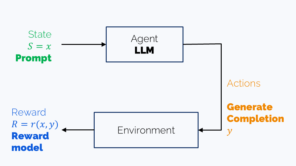
An LLM may be considered as an agent in a single-turn game which terminates after the completion is created. In this case, we have the following components:

• An agent: that is, our LLM,
• An observed state: the prompt
• Actions: generation of a completion
• Reward: might be a reward model score or an “answer is correct” reward

In complex agentic scenarios, such as web shopping, generating one completion becomes a single step a longer game, which may involve many iterations until the task is accomplished. The state also becomes richer and includes observations from the apps used. The actions are, strictly speaking, still the possible completions, including tool calls.

Reinforcement Learning strategies might be classified along several axes:

• Learning goal, as discussed earlier, including alignment, long-reasoning capabilities etc.
• Learning tactics, including PPO, DPO, GRPO, DAPO etc. We’ll discuss them in details further in this long read.
• Reward types, including:
  • Explicit (rule-based) rewards such as answer accuracy, format correctness, or success in performing a web shop task. They are used for training long reasoners and components of agentic systems.
  • Trainable rewards. These are used when rule-based scoring is impossible. For example, scoring helpfulness of a dialog or harmlessness of bot’s answers requires training a reward model. We’ll discuss training methodology in the respective section.
  • “Intrinsic reward”, which is actually used to replace RL by SFT. We’ll talk about it in the DPO section.

Note. The term “RLHF” (Reinforcement Learning with Human Feedback) historically refers to alignment training with a reward model, which is trained on human-annotated data (hence human feedback).

In this long read, we’ll discuss most notable RL strategies used to train LLMs. We’ll focus on the single-turn scenario of alignment / long reasoning training; this will make things easier for us and allow to avoid pressing a whole RL course into one text. At the same time, we won’t be shy with math, so read with caution.

---

In a general, multi-turn case, there is another important distinction between:

• outcome reward, which is only assigned at the end of a trajectory
• process reward, which is assigned for each action (or some action group)

If we consider an LLM’s generation as a multi-turn game, where each turn is generation of a single token, the completion-wise reward we discussed earlier becomes an outcome reward, while a process reward would score partial completions after each generated token.

Part 1. Reward model training

A reward model $r(x, y)$ measures how much a completion $y$ is “appropriate” for a prompt $x$. Being “appropriate” might mean many things, depending on our training goals. It may encompass:

• Whether an LLM exhibits bias - a systematic, specific treatment of certain groups of people or, more broadly, objects or phenomena. An example of bias is an image generation model that only generates men when prompted by “A portrait of a CTO”.
• Whether an LLM is harmless - can it be provoked to generate abusive, toxic, or explicit content?
• Whether an LLM’s answers are helpful.

The reward is a ranking model. Its meaning is: if $r(x, y) > r(x, y’)$, then $y$ is a more appropriate completion than $y’$.

CAUTION: It is not a classification model. It doesn’t say “this is good, that is bad” (not in a typical situation, at least). Even for two good completions, it allows to say which is better.

Training strategy depends on what kind of data we are able to collect. As in any ranking task, there are three main types of data:

• Pairwise. That is, we train the model on triplets $(x, y_a, y_r)$, where where $y_a$ is more appropriate than $y_r$. In other words, the data is “Completion $y_a$ is more appropriate than Completion $y_r$ for the prompt $x$”. Typical RLHF/DPO fine tuning consumes this very type of data, and the other two types are way more niche. The reward model is trained by minimizing \(\mathcal{L}_{RM} = -\mathbb{E}_{(x, y_a, y_r)\sim\mathcal{D}}\log\sigma(r(x, y_a) - r(x, y_r)),\) where $\mathbb{E}_{(x, y_a, y_r)\sim\mathcal{D}}$ means in practice: “average over a batch of triplets sampled from the whole dataset $\mathcal{D}$”.

If you want to understand this loss better, check the next subsection (Terry-Bradley model).

• Pointwise. It uses data like “thumbs up/down for this completion” of “Five stars for this completion”. A reward model for this could be trained for ordinary classification or regression task, or rather you can use an intrinsic reward function. Pointwise reward is a rare choice, but you can check the KTO (Kahneman-Tversky optimization) paper for an example.

• Listwise. The data is like “Completion $y_1$ is better than completion $y_2$ which is better than completion $y_3$ and so on”. It is possible to collect such data with ChatGPT or other powerful LLMs. This kind of data isn’t very popular either; for an example, check Starling-7B.

Note: RLHF vs RLAIF. Traditionally, data for reward model training is labeled with human annotators. An example pipeline might be:

1. A number of prompts is chosen
2. For each prompt, several completions (say, 5 or 7) are generated
3. For each prompt, human annotators rank all the completions
4. The best ranking completion is labeled as chosen; the worst ranking is labeled as rejected. All other completions are discarded.

Due to involvement of humans in the data labeling process, RLHF is called Reinforcement Learning with Human Feedback. In most cases, top LLM creators indeed try to employ humans in order to incorporate real human preference into the reward model.

However, human labelers aren’t cheap, so in some cases already-trained high-quality LLMs are used to score completions. If that’s the case, RL training gets the name RLAIF (Reinforcement Learning with AI feedback). This way, in a sense, the completion-labeling LLM is distilled into the reward model and, through it, into the new, RLAIF-trained LLM.

Bradley-Terry model

Math warning

The Bradley-Terry model was created as a ranking model. Imagine, for example, that several teams compete in a championship and we want to make a total ranking of the teams. We can do it by assigning to the $i$-th team a numerical measure $\beta_i$ of its strength. Ideally, the outcome of a competition between teams $i$ and $j$ should be determined by $\beta_i - \beta_j$.

The Bradley-Terry model treats the outcome of a game between teams $(i, j)$ as a Bernoulli random variable with probability of $i$ winning equal to

\(p^*(team_i\succ team_j) = \sigma(\beta_i - \beta_j) = \frac{1}{1 + e^{-(\beta_i - \beta_j)}} =\) \(=\frac{e^{\beta_i - \beta_j}}{1 + e^{\beta_i - \beta_j}} = \frac{e^{\beta_i}}{e^{\beta_i} + e^{\beta_j}}\)

Simply put, it’s our usual way of making $\beta_i - \beta_j$ into probabilities of winning, such that going $team_i\succ team_j\longleftrightarrow team_j\succ team_i$ is made by sign change $\beta_i - \beta_j \longleftrightarrow \beta_j - \beta_i$:

\[p^*(team_j\succ team_j) = 1 - \sigma(\beta_i - \beta_j) = \sigma(\beta_j - \beta_j)\]

During LLM training we work with user preferences in the form “for a prompt $x$ the completion $y_a$ is better than $y_r$” (a and r stand for “accepted” and “rejected”).

We model the strength of a completion $y$ of a prompt $x$ by the reward model value $r^*(x, y)$. The formulas above become:

\[p^*(y_a\succ y_r | x) = \sigma(r^*(x, y_a) - r^*(x, y_r))\]

The reward model is trained by negative loglikelihood optimization:

\[\mathcal{L}_{RM} = -\mathbb{E}_{(x, y_a, y_r)\sim\mathcal{D}}\log\sigma(r^*(x, y_a) - r^*(x, y_r)),\]

where $(x, y_a, y_r)\sim\mathcal{D}$ stands for sampling from the dataset that we were lucky to collect. So, $\mathbb{E}_{(x, y_a, y_r)\sim\mathcal{D}}$ stands in practice for “average over all $(x, y_a, y_r)$ from the dataset $\mathcal{D}$” or “average over all $(x, y_a, y_r)$ in a batch sampled from the dataset $\mathcal{D}$”.

Part 2. PPO

PPO (Proximal Policy Optimization) was the algorithm used in the original RLHF for creation of InstructGPT from GPT-3. Up to some tweaks, it’s still used now despite the rise of GRPO. In this section, we’ll try to explain what motivated PPO’s quite complicated loss function.

Caution. We will only discuss a single-turn setup, as in RLHF or long-reasoner training. But keep in mind that PPO can be used in general case as well - for example to train an LLM for multi-turn agentic scenarios. If you want to learn what PPO looks like in general case, please check some full RL course, or this post by Lilian Weng, or OpenAI’s introduction to RL.

---

To start with, we have a certain reward function $r(x, y)$ ($x$ is a prompt and $y$ is its completion). It may be a trained reward function that scores helpfullness/harmlessness or a detetministic one, like final answer correctness. Anyway, it should be fixed during RL training — in RLHF, the reward model is trained before RL starts.

Some notations:

• Starting from now, we’ll be denoting our LLM by $\pi_{\theta}(y\vert x)$ and calling it policy to match the traditional RL terminilogy. But don’t be afraid: it’s just our good old LLM with parameters $\theta$ that predicts completion $y$ given a prompt $x$ or, more generally, probabilities of completions $y$ given $x$.
• We take a dataset of prompts $\mathcal{D} = {(x)}$. Yes, no completions now;

• We want to maximize the reward $r(x, y)$ of generated $y$ in pursuit of making the LLM give us more rewarding completions: \(\mathbb{E}_{x\sim\mathcal{D}, y\sim\pi_{\theta}(y\vert x)}r(x, y)\longrightarrow\max\limits_{\theta}.\) Here,

  \[\mathbb{E}_{x\sim\mathcal{D}, y\sim\pi_{\theta}(y\vert x)}\]

  techincally describes the following process:

  1. We sample a batch of prompts from $\mathcal{D}$
  2. For each prompt, we generate a completion $y$ using the current LLM $\pi_{\theta}$ (yes, the one we’re training, and it changes during training)
  3. We score each pair $(x, y)$ with the reward model $r$
  4. We average rewards in the batch

Step 1. The reward is not the loss

Now, we would love to say that $y = \pi_{\theta}(y\vert x)$ and we’re just maximizing $r(x, \pi_{\theta}(y\vert x))$, but that’s not true. The problem is that $\pi_{\theta}(y\vert x)$ is not a function, because it involves token sampling. The right way of putting it is $y = \pi_{\theta}(y\vert x)$; this is a stochastic procedure, and we can’t just differentiate through it and optimize $r$ with gradient descent.

We’ll be able to overcome this obstacle through math. Let’s recall the actual loss function:

\[\mathbb{E}_{x\sim\mathcal{D}, y\sim\pi_{\theta}(y\vert x)}r(x, y)=\] \[\mathbb{E}_{x\sim\mathcal{D}}\,\mathbb{E}_{y\sim\pi_{\theta}(y\vert x)}r(x, y)\]

At this point it’s useful to recall the definition of mathematical expectation, rewriting it as

\[\mathcal{L} = \frac1{|D|}\sum_{x\sim\mathcal{D}}\,\sum_{y}\pi_{\theta}(y\vert x)r(x, y)\]

Here, we treat $\pi_{\theta}(y\vert x)$ as the probability of $y$ given $x$, as predicted by $\pi_{\theta}$.

Step 2. Policy gradient

Since we want to optimize the loss with stochastic gradient descent (or, more accurately, some of its modifications such as Adam), we need to actually find $\nabla_{\theta}\mathcal{L}$. Moreover, we want to estimate the gradient using not the whole dataset, but rather a batch sampled from it.

We’ll start by recalling how this works for usual loss functions, and then we’ll understand what’s wrong with ours. In supervised tasks (classification, regression, etc), we have, for a model $h_{\phi}(z)$ with parameters $\phi$, a loss

\[\mathcal{G} = \mathbb{E}_{z\in Z}G(h_{\phi}(z)) = \frac{1}{|Z|}\sum_{z\in Z}G(h_{\phi}(z))\]

(Here, $\frac{1}{\vert Z\vert}\sum$ might become $\int$ if we assume that the dataset is infinite.)

The gradient is

\[\nabla_{\phi}\mathcal{G} = \frac{1}{|Z|}\sum_{z\in Z}\nabla_{\phi}G(h_{\phi}(z)) = \mathbb{E}_{z\in Z}G(h_{\phi}(z))\]

Now, given a batch $B\subset Z$, we can estimate this mathematical expectation as

\[\mathbb{E}_{z\in Z}G(h_{\phi}(z)) \approx \frac1{|B|}\sum_{z\in B}\nabla_{\phi}G(h_{\phi}(z)),\]

which gives us exactly the familiar stochastic gradient descent.

Now, let’s find the derivative of $\nabla_{\theta}\mathcal{L}$:

\[\nabla_{\theta}\mathcal{L} = \nabla_{\theta}\frac1{|D|}\sum_{x\sim\mathcal{D}}\,\sum_{y}\pi_{\theta}(y\vert x)r(x, y) =\] \[=\frac1{|D|}\sum_{x\sim\mathcal{D}}\,\sum_{y}\left[\nabla_{\theta}\pi_{\theta}(y\vert x)r(x, y)\right]\]

Now, to estimate this gradient on a batch of prompts $x$, we need to write this down as

\[\mathbb{E}_{x\sim\mathcal{D}}\,\mathbb{E}_{y\sim\pi_{\theta}(y\vert x)}(\text{something}) = \frac1{|D|}\sum_{x\sim\mathcal{D}}\,\sum_{y}\pi_{\theta}(y\vert x)\cdot[\text{something}],\]

But how?!

Well, let’s do a very naive transformation:

\[\frac1{|D|}\sum_{x\sim\mathcal{D}}\,\sum_{y}\nabla_{\theta}\pi_{\theta}(y\vert x)r(x, y) =\] \[= \frac1{|D|}\sum_{x\sim\mathcal{D}}\,\sum_{y}\nabla_{\theta}\pi_{\theta}(y\vert x)\cdot \frac{\pi_{\theta}(y\vert x)}{\pi_{\theta}(y\vert x)}r(x, y)\]

Luckily, $\frac{\nabla_{\theta}\pi}{\pi} = \nabla_{\theta}\log{\pi}$, so we can rewrite this as:

\[= \frac1{|D|}\sum_{x\sim\mathcal{D}}\,\sum_{y}\pi_{\theta}(y\vert x)\cdot \nabla_{\theta}\log\pi_{\theta}(y\vert x)r(x, y) = \mathbb{E}_{x\sim\mathcal{D}}\,\mathbb{E}_{y\sim\pi_{\theta}(y\vert x)}\log\pi_{\theta}(y\vert x)r(x, y)\]

Now, given a batch of prompts $B$, we can estimate the gragient as

\[\frac1{|D|}\sum_{x\sim\mathcal{D}, y\sim\pi_{\theta}(y\vert x)}\,\nabla_{\theta}\log\pi_{\theta}(y\vert x)r(x, y)\]

Note that we actually estimated the internal mathematical expectation

\[\mathbb{E}_{y\sim\pi_{\theta}(y\vert x)}[\ldots]\]

with just one point. This makes the estimate not very accurate, but at least theoretically unbiased.

Step 3. Advantage

The formulas here are only valid for the single-turn setup (outcome reward)

Though the gradient estimate we’ve produced is unbiased, it is still very noisy, with high variance. A common practice is replacing the reward in the loss with the advantage functon

\[\widehat{A}(x, y) = r(x, y) - \widehat{V}_{\phi}(x),\]

where $\widehat{V}_{\phi}(x)$ is an estimate of the average reward of $r(x, y)$, trained alongside the policy as a separate LLM’s “value head” with the loss

\[\frac1{|B|}\sum_{x\in B, y\sim\pi_{\theta}(y\vert x)}\left(\widehat{V}_{\phi}(x) - r(x, y)\right)^2\]

The cool fact about advantage is that

\[\nabla_{\theta}\mathbb{E}_{x\sim\mathcal{D}}\,\mathbb{E}_{y\sim\pi_{\theta}(y\vert x)}\log\pi_{\theta}(y\vert x)\widehat{A}(x, y) =\] \[\nabla_{\theta}\mathbb{E}_{x\sim\mathcal{D}}\,\mathbb{E}_{y\sim\pi_{\theta}(y\vert x)}\log\pi_{\theta}(y\vert x)r(x, y) - \nabla_{\theta}\mathbb{E}_{x\sim\mathcal{D}}\,\mathbb{E}_{y\sim\pi_{\theta}(y\vert x)}\log\pi_{\theta}(y\vert x)\widehat{V}(x) =\] \[\nabla_{\theta}\mathbb{E}_{x\sim\mathcal{D}}\,\mathbb{E}_{y\sim\pi_{\theta}(y\vert x)}\log\pi_{\theta}(y\vert x)r(x, y) - \nabla_{\theta}\mathbb{E}_{x\sim\mathcal{D}}\,\widehat{V}(x)\underbrace{\mathbb{E}_{y\sim\pi_{\theta}(y\vert x)}\log\pi_{\theta}(y\vert x)}_{=1} =\] \[\nabla_{\theta}\mathbb{E}_{x\sim\mathcal{D}}\,\mathbb{E}_{y\sim\pi_{\theta}(y\vert x)}\log\pi_{\theta}(y\vert x)r(x, y) - \nabla_{\theta}\mathbb{E}_{x\sim\mathcal{D}}\,\widehat{V}(x)\underbrace{\mathbb{E}_{y\sim\pi_{\theta}(y\vert x)}\log\pi_{\theta}(y\vert x)}_{=1} =\] \[\nabla_{\theta}\mathbb{E}_{x\sim\mathcal{D}}\,\mathbb{E}_{y\sim\pi_{\theta}(y\vert x)}\log\pi_{\theta}(y\vert x)r(x, y) - 0\]

That is, replacing $r(x, y)$ by $\widehat{A}(x, y)$ doesn’t change the gradient of the loss. At the same time, it can be proved that it decreases the gradient’s variance. (Actually, $\widehat{V}_{\phi}(x)$ is, in a sense, the “optimal” thing we can subtract from $r(x,y)$ in order to reduce the gradient’s variance.) We’ll omit the mathematical proof here, highlighting instead the common sense behind the advantage function.

Imagine that we’re solving the alignment problem with RL. Imagine also that at some point in training the LLM generates a very toxic completion $y$ which brings a very low reward $r(x, y)$. Our initial loss would punish the model uniformly, whatever the initial $x$ could be. But the new strategy is more wise: it compares $r(x, y)$ with the expected reward given that $x$. So:

• If the prompt itself is toxic and manipulative, $\widehat{V}_{\phi}(x)$ is likely low, and we won’t punish the model too harsh for low $r(x, y)$.
• On the other hand, if the prompt is quite innocent, $\widehat{V}_{\phi}(x)$ is likely high, and it’s only reasonable to strictly penalize the model for completions that score far beyond mean expected reward for the prompt $x$.

Step 4. Importance sampling

The loss

\[\mathbb{E}_{x\sim\mathcal{D}}\,\mathbb{E}_{y\sim\pi_{\theta}(y\vert x)}\widehat{A}(x, y) \approx \frac1{|B|}\sum_{y}\pi_{\theta}(y\vert x)\widehat{A}(x, y)\]

is the function of the policy $\pi_{\theta}(y\vert x)$. Roughly putting, the loss tells us which policies $\pi_{\theta}(y\vert x)$ are better and which is worse. But the thing is — the completions $y$ are generated not from this variable policy $\pi_{\theta}(y\vert x)$, but from the very concrete and fixed policy — let’s call it $\pi_{\text{old}}(y\vert x)$. This makes the whole formula wrong; the right one should be

\[\mathbb{E}_{x\sim\mathcal{D}}\,\mathbb{E}_{\mathbf{y\sim\pi_{old}(y\vert x)}}[\text{something}]\]

But how can we change

\[\mathbb{E}_{y\sim\pi_{\theta}(y\vert x)}\]

into

\[\mathbb{E}_{y\sim\pi_{\text{old}}(y\vert x)}?\]

Luckily, this can be done through a trick otherwise known as importance sampling:

\[\frac1{|B|}\sum_{y}\pi_{\theta}(y\vert x)\widehat{A}(x, y) = \frac1{|B|}\sum_{y}\pi_{\theta}(y\vert x)\cdot\mathbf{\frac{\pi_{old}(y\vert x)}{\pi_{old}(y\vert x)}}\cdot\widehat{A}(x, y) =\] \[= \frac1{|B|}\sum_{y}\pi_{\text{old}}(y\vert x)\cdot\frac{\pi_{\theta}(y\vert x)}{\pi_{\text{old}}(y\vert x)}\widehat{A}(x, y) =\] \[\mathbb{E}_{x\sim\mathcal{D}}\,\mathbb{E}_{\mathbf{y\sim\pi_{old}(y\vert x)}}\frac{\pi_{\theta}(y\vert x)}{\pi_{\text{old}}(y\vert x)}\widehat{A}(x, y) =: \mathcal{L}\]

This change brings yet another benefit. Let’s understand what it is.

If we change the policy after each batch - which is unlikely to be spectacularly large - and sample new completions from the new model, it seems like we’re doing two changes at a time: parameter update + data sampling process update. That might be a bit too rapid; we might loose control over the training process. A milder strategy would be to sample a larger batch from $\pi_{old}(y\vert x)$ and then to make several batch-gradients steps (with smaller batches) on this data, before replacing $\pi_{old}(y\vert x)$ by the updated policy. This might make the training process smoother. And indeed, in practice $\pi_{old}(y\vert x)$ lasts not for a single batch but for a certain training epoch.

Step 5. Reward hacking and KL regularization

If you get too carried away with maximizing reward (human preferences), you can ruin the quality. An absurd, but illustrative example: a model that politely refuses to answer any question is perfectly non-toxic, although completely useless. Situations, when the model learns to increase reward at all costs, eventually harming the actual goal behind the reward, are known as reward hacking.

To counter reward hacking, it’s good to prevent the LLM from drifting too far away during RL training. There are several ways of establishing this; the most popular are KL penalty and clipped objective. We’ll start with the first one.

The idea of the TRPO (Trust Region Policy Optimization) approach is to directly ensure that the predicted token probability distribution $\pi_{\theta}(y\vert x)$ doesn’t get far from its intial state $\pi_{\text{ref}}$ (reference policy).

The most common tool for measuring distance between distributions is KL-divergence. So, the regularized version of the training objective is:

\[\begin{cases} \mathbb{E}_{x\sim\mathcal{D}}\,\mathbb{E}_{\mathbf{y\sim\pi_{old}(y\vert x)}}\frac{\pi_{\theta}(y\vert x)}{\pi_{\text{old}}(y\vert x)}\widehat{A}(x, y)\longrightarrow\max\\ \mathbb{D}_{\mathrm{KL}}\left[\pi_{\theta}(y \vert x)||\pi_{\text{ref}}(y \vert x)\right]\leqslant\delta \end{cases}\]

This task can be solved directly with a variety of constrained optimization methods. However in practice just a regularized objective is used:

\[\mathcal{L} = \mathbb{E}_{x\sim\mathcal{D}}\,\mathbb{E}_{\mathbf{y\sim\pi_{old}(y\vert x)}}\frac{\pi_{\theta}(y\vert x)}{\pi_{\text{old}}(y\vert x)}\widehat{A}(x, y) - \beta\mathbb{D}_{\mathrm{KL}}\left[\pi_{\theta}(y \vert x)||\pi_{\text{ref}}(y \vert x)\right]\]

Note 1: This objective is being maximized. So, the KL summand here is minimized.

Note 2: Having both $\pi_{\text{old}}$ and $\pi_{\text{ref}}$ in one formula might be confusing, but it’s two different policy snapshots:

• $\pi_{\text{old}}$ is the pre-current-epoch policy.
• $\pi_{\text{ref}}$ is the initial, pre-RL policy.

Note 3: KL-divergence is outside

\[\mathbb{E}_{x\sim\mathcal{D}}\,\mathbb{E}_{\mathbf{y\sim\pi_{old}(y\vert x)}}.\]

If we want to drag it inside, we will use the definition of KL-divergence

\[\mathbb{D}_{\mathrm{KL}}(p||q) = \sum_i p_i\log\frac{p_i}{q_i} = \mathbb{E}_p\log\frac{p}{q}\]

and write instead

\[\mathcal{L} = \mathbb{E}_{x\sim\mathcal{D}}\, \mathbb{E}_{y\sim\pi_{\text{old}}(y\mid x)} \left[ \frac{\pi_{\theta}(y\mid x)}{\pi_{\mathrm{old}}(y\mid x)} \,\widehat{A}(x, y) \right] \;-\; \beta\, \mathbb{D}_{\mathrm{KL}}\!\bigl[\pi_{\theta}(y\mid x)\,\big\|\,\pi_{\mathrm{init}}(y\mid x)\bigr] \;-\; \beta\, \log\frac{\pi_{\theta}(y\mid x)}{\pi_{\mathrm{init}}(y\mid x)}.\]

Note 4: The original InstructGPT paper also suggesting adding one more summand to the objective to directly control performance on the pretraining dataset:

\[\mathcal{L} = \mathbb{E}_{x\sim\mathcal{D}} \mathbb{E}_{y\sim\pi_{\mathrm{old}}(y\mid x)} \left[ \frac{\pi_{\theta}(y\mid x)}{\pi_{\mathrm{old}}(y\mid x)} \,\widehat{A}(x, y) - \beta \log\frac{\pi_{\theta}(y\mid x)}{\pi_{\mathrm{init}}(y\mid x)} \right] +\] \[+ \gamma\mathbb{E}_{x\sim\mathbb{D}_{\text{pretrain}}}\log\pi_{\theta}(x)\]

Step 6. Clipped Surrogate Objective

KL-divergence in not the only possible mechanism to control the drift of $\pi_{\theta}(y\vert x)$ from initial policy. Clipped Surrogate Objective aims to prevent extreme updates during gradient descent instead of imposing global regularization.

The idea is as follows. As we maximize

\[\frac1{|B|}\sum_{x\in B, y\sim\pi_{\theta}(y\vert x)}\frac{\pi_{\theta}(y\vert x)}{\pi_{\text{old}}(y\vert x)}\widehat{A}(x, y),\]

for a given batch $B$, both advantages and the old policy are fixed, so we can only change $\pi_{\theta}(y\vert x)$. Under such conditions, ideally $\pi_{\theta}(y\vert x)$ should

• become $1$ for $(x, y)$ with $\widehat{A}(x, y) > 0$ and
• become $0$ for $(x, y)$ with $\widehat{A}(x, y) < 0$.

And it should occur as quickly as it can - which means potentially large gradients and drastic changes in the parameters $\theta$. (Length of the gradient = speed of change.)

To prevent this from happening, let’s discourage $\pi_{\theta}(y\vert x)$ from going far from $\pi_{\text{old}}(y\vert x)$ inside one epoch by clipping the importance sampling ratio:

\[\frac1{|B|}\sum_{x\in B, y\sim\pi_{\theta}(y\vert x)}\,\text{clip}\left(\frac{\pi_{\theta}(y\vert x)}{\pi_{\text{old}}(y\vert x)}, 1 - \varepsilon, 1 + \varepsilon\right)\widehat{A}(x, y),\]

Here, $\varepsilon$ is a hyperparameter, which can typically be 0.2.

A reminder. Clipping does the following:

\[\text{clip}(r, 1 - \varepsilon, 1 + \varepsilon) = \begin{cases} 1 - \varepsilon,\ r < 1 - \varepsilon,\\ r,\ 1 - \varepsilon \leqslant r < 1 + \varepsilon,\\ 1 + \varepsilon,\ r \geqslant 1 + \varepsilon \end{cases}\]

So, basically, clipping stops $\pi_{\theta}(y\vert x)$ from being updated as soon as it goes far enough from the old policy — also defining a trust region of sorts.

However, we don’t want our objective to become larger than it was before. Indeed, we maximize $\mathcal{L}$, and if our manipulations increase it, we’re making ourself overly optimistic. So, it’s common to take minimum between the initial and the clipped loss:

\[\mathcal{L} = \mathbb{E}_{x\sim\mathcal{D}}\,\mathbb{E}_{\mathbf{y\sim\pi_{old}(y\vert x)}}\min\left[\frac{\pi_{\theta}(y\vert x)}{\pi_{\text{old}}(y\vert x)}\widehat{A}(x, y), \text{clip}\left(\frac{\pi_{\theta}(y\vert x)}{\pi_{\text{old}}(y\vert x)}, 1 - \varepsilon, 1 + \varepsilon\right)\widehat{A}(x, y)\right]\]

This one is Clipped Surrogate Objective. It can be used with KL regularizer term, but often the KL penalty is omitted.

And that’s it!

Indeed, the loss we’ve written above is the most common formulation of PPO for a single-turn game.

Per-token objective

So far, we considered an RL setup where the agent (an LLM) produces the whole completion as a single action - and is rewarded only for its final result. However, in many cases per-token setup is considered, where an action is generation of a single token. In this case, the reward is calculated for every prefix $y_{\leqslant t}$ of a completion $y$, and the objective features another sum - over $t$:

\[\mathcal{L} = \mathbb{E}_{x\sim\mathcal{D}}\,\mathbb{E}_{\mathbf{y_{\leqslant t}\sim\pi_{old}(y\vert x)}}\min\left[\frac{\pi_{\theta}(y_t\vert x, y_{<t})}{\pi_{\text{old}}(y_t\vert x, y_{<t})}\widehat{A}_t(x, y_{< t}, y_t), \text{clip}\left(\frac{\pi_{\theta}(y_t\vert x, y_{<t})}{\pi_{\text{old}}(y_t\vert x, y_{<t})}, 1 - \varepsilon, 1 + \varepsilon\right)\widehat{A}_t(x, y_{< t}, y_t)\right] \approx\] \[\approx \frac{1}{|B|}\sum_{x\in B, y\sim\pi_{old}(y\vert x)}\,\frac1{\text{len}(y)}\sum_{t=1}^{\text{len}(y)}\,\min\left[\dots\right]\]

This formula looks more or less the same as its single-turn counterpart, but the actual difference hides inside the advantage function $\widehat{A}_t$.

In multi-turn setup, it’s a more complicated thing. Without going into details, we’ll say that

\[\widehat{A}_t(\underbrace{[x, y_{< t}]}_{\text{state}}, \underbrace{y_t}_{\text{action}}) = Q_t([x, y_{< t}], y_t) - V_t([x, y_{< t}]),\]

where

• $V_t([x, y_{< t}])$ is smth like the expected cumulative reward we can get, if we start with $[x, y_{< t}]$ and generate further tokens with $\pi_{\theta}$. As before, it is predicted by a trained value head.
• $Q_t([x, y_{< t}], y_t)$ is smth like the expected cumulative reward we can get, if we start with $x, y_{< t}$, then choose $y_t$ as the next token and, after that, generate further tokens with $\pi_{\theta}$. There are different ways of calculating it. Probably the most popular is the 1-step lookahead

\[Q_t\bigl([x,\;y_{<t}],\;y_t\bigr) \;\approx\; r\bigl(x,\;y_{\leqslant t}\bigr) \;+\; \gamma\, V_{t+1}\bigl([x,\;y_{\leqslant t+1}]\bigr).,\]

where $0 < \gamma < 1$ is a hyperparameter.

Quite often though, a more sophisticated Generalized Advantage Estimation is used:

\[\widehat{A}^{\text{GAE}}_t([x, y_{< t}], y_t) = \sum_{l=0}^{\infty}(\gamma\lambda)^l\delta_{t+l},\]

where $0 < \lambda < 1$ is yet another hyperparameter and

\[\delta_l = r(x, y_{\leqslant l}) ​+ \gamma V_{l+1}([x, y_{\leqslant l}]) - V_l([x, y_{<l}])\]

This was sketchy, of course. If you want to truly understand these formulas, please consider taking a full RL course.

GRPO

Group Relative Policy Optimization (GRPO) became a fashionable alternative to PPO since it was used to train DeepSeek-R1 from DeepSeek-V3 for long reasoning. The main difference between PPO and GPRO is that GRPO doesn’t use value head $V$. Instead, it employs batch-size relative advantage. Here’s how it works (we use notation from the paper):

• For a prompt $q$, several completions $o_1,\ldots,o_G$ are generated.
• For every completion, its reward $r_i = r(q, o_i)$ is computed.

• Then, the relative advantage is calculated by normalizing the reward:

  \[\widehat{A}_{i} = \frac{r_i - \textrm{mean}(r_1,\ldots,r_G)}{\textrm{std}(r_1,\ldots,r_G)}\]

  Like the trained value head in PPO, this helps to reduce variance of gradients.

• The authors of DeepSeek-R1 suggested to use both \textbf{Clipped surrogate objective} and KL-regulatization:

  \[\mathcal{L}(q) = \frac1G\sum_{i=1}^G\left[\min\left(\frac{\pi_{\theta}(o_i\mid q)}{\pi_{\mathrm{old}}(o_i\mid q)}\widehat{A}_{i}, \mathrm{clip}\left(\frac{\pi_{\theta}(o_i\mid q)}{\pi_{\mathrm{old}}(o_i\mid q)}; 1 - \varepsilon, 1 + \varepsilon\right)\widehat{A}_{i}\right) - \beta\mathbb{D}_{\mathrm{KL}}(\pi_{\theta}\|\pi_{\text{ref}})\right]\]

• The final loss is

  \[\mathbb{E}_{q\sim\mathcal{D},\,o_i\sim\pi_{\theta}(o\mid q)}\mathcal{L}\]

  That is, $q$ is sampled from the data and $o_i$ from the policy (LLM) $\pi_{\theta}$ that we are training.

This loss also has its per-token version.

DAPO

As GRPO gained popularity, its efficiency came under scrutiny, leading to a number of suggested enhancements. We’ll discuss the DAPO paper by ByteDance, which shares insights about the sources of potential problems of per-token GRPO and offers some remedies, packed into the Dynamic sAmpling Policy Optimization (DAPO) strategy.

First of all, let’s write down the per-token GRPO loss:

\[\mathcal{L}(q) = \frac1G\sum_{i=1}^G\frac1{|o_i|}\sum_{t=1}^{|o_i|}\left[\min\left(\frac{\pi_{\theta}(o_{i,t}\mid q,o_{i,< t})}{\pi_{\mathrm{old}}(o_{i,t}\mid q,o_{i,< t})}\widehat{A}_{i, t}, \mathrm{clip}\left(\frac{\pi_{\theta}(o_{i,t}\mid q,o_{i,< t})}{\pi_{\mathrm{old}}(o_{i,t}\mid q,o_{i,< t})}; 1 - \varepsilon, 1 + \varepsilon\right)\widehat{A}_{i, t}\right) - \beta\mathbb{D}_{\mathrm{KL}}(\pi_{\theta}\|\pi_{\text{ref}})\right],\]

where $r_{i, t} = r(q, o_{i, \leqslant t})$ and

\[\widehat{A}_{i, t} = \frac{r_{i, t} - \textrm{mean}(r_{1, t},\ldots,r_{G, t})}{\textrm{std}(r_{1, t},\ldots,r_{G, t})}\]

And the first thing that ByteDance suggested was to ditch the KL summand. (Which sounds reasonable, because clipping and KL have the same goal.)

• Entropy collapse phenomenon. The authors observe that policy’s entropy tends to decrease rapidly as training progresses. This might be attributed to the GRPO’s clipping mechanism:

  \[\text{clip}\left(\frac{\pi_{\theta}(o_i|q)}{\pi_{\text{old}}(o_i|q)}; 1 - \varepsilon; 1 + \varepsilon\right)\]

  Here, $\pi_{\theta}(o_i\vert q)$ can only meaningfully vary between $\pi_{\text{old}}(o_i\vert q)\cdot(1 - \varepsilon)$ and $\pi_{\text{old}}(o_i\vert q)(1 + \varepsilon)$. If $\pi_{\text{old}}(o_i\vert q)$ is small for a token $o_i$, the loss function gives “insufficient motivation” for $\pi_{\theta{old}}(o_i\vert q)$ to increase. This might lead to the situation where high-probability tokens get their probabilities further boosted, while low-probability ones fade away. This can lead to a less diverse policy.

  The authors propose a Clip-Higher strategy, raising the clipping ceiling and thus allowing low-probability tokens to gain more traction:

  \[\text{clip}\left(\frac{\pi_{\theta}(o_i|q)}{\pi_{\text{old}}(o_i|q)}; 1 - {\color{red}\varepsilon_{\text{low}}}; 1 + {\color{red}\varepsilon_{\text{high}}}\right)\]

• Optimization paralysis at rewards close to 1. When the reward, which typically ranges between 0 and 1, becomes very close to 1, the relative advantage term in GRPO, $\widehat{A}_{i,t}$, approaches $0$ because of the normalization. This significantly diminishes the optimization signal, making it difficult for the model to learn further improvements. The same issue also arises if all accuracies within a batch are close to zero.

  The authors suggest to over-sample and filter out prompts with rewards equal to 1 and 0. This is exactly the Dynamic Sampling that gave the name to DAPO.

• Low importance of individual tokens in long completions. Since clipped advantages are averaged across the sequence, - $\frac1{\vert o_i\vert }\sum_{i=1}^{\vert o_i\vert}$ - the contribution of any individual token’s reward becomes less significant.

  The authors suggest averaging the advantages across the whole batch:

  \[\frac1G\sum_{i=1}^G\frac1{|o_i|}\sum_{i=1}^{|o_i|} \quad \mapsto \quad \frac1{G\sum_{i=1}^{G}|o_i|}\sum_{i=1}^G\sum_{t=1}^{|o_i|}\]

• Inadequate punishment of long outputs. In RL training, overlong samples are often truncated. But if we train long reasoners, this might backfire, because we’ll be punishing long but potentially correct solutions. DAPO suggests addressing this by masking truncated sequences from loss computation and introducing a soft, linear punishment for overlong outputs.

DPO

Reinforcement learning in general is notorious for instability, so researchers sought for ways of removing RL from RLHF.

One of the most successful options so far is Direct preference optimization suggested in the NeurIPS 2023 best paper award winning Your Language Model is Secretly a Reward Model paper. Its main idea is that we don’t need to train an external reward model and we can find it inside our LLM. Let’s see how it’s done.

Analytical solution for RLHF objective maximization

The authors showed that maximum of the RLHF loss can be found analytically, at least of the following version of it (no clipping, no importance sampling, no advantages, but with the KL penalty):

\[\mathcal{L}_{\text{RLHF}} = \mathbb{E}_{x\sim\mathcal{D}, y\sim\pi_{\theta}(y \vert x)}\left[r(x, y) - \beta\log\frac{\pi_{\theta}(y \vert x)}{\pi_{\text{ref}}(y \vert x)}\right]\] \[=-\mathbb{E}_{x\sim\mathcal{D}, y\sim\pi_{\theta}(y \vert x)}\left[\log\frac{\pi_{\theta}(y \vert x)}{\pi_{\text{ref}}(y \vert x)\exp\left(\frac1{\beta}r(x, y)\right)}\right]\\\]

The expression

\[-\mathbb{E}_{x\sim\mathcal{D}, y\sim\pi_{\theta}(y \vert x)}\log\frac{\pi_{\theta}(y \vert x)}{\text{something}}\]

resembles

\[-\mathbb{D}_{\mathrm{KL}}(\pi_{\theta}(y \vert x)||\text{something}).\]

If it were so, its maximum, i.e. the minimum of KL-divergence would be when something coincides with $\pi_{\theta}(y\vert x)$.

The only problem is that $\pi_{\text{ref}}(y \vert x)\exp\left(\frac1{\beta}r(x, y)\right)$ is not guaranteed to be a probabilistic distribution. That is, it probably doesn’t sum to $1$. Let’s denote

\[Z(x) = \sum_y\pi_{\text{ref}}(y \vert x)\exp\left(\frac1{\beta}r(x, y)\right)\] \[\pi^*(y \vert x) = \frac1{Z(x)}\pi_{\text{ref}}(y \vert x)\exp\left(\frac1{\beta}r(x, y)\right)\]

and rewrite

\[\mathcal{L}_{\mathrm{RLHF}} =\mathbb{E}_{x\sim\mathcal{D}, y\sim\pi_{\theta} (y \vert x)}\left[\log{Z}(x) - \log\frac{\pi_{\theta}(y \vert x)}{\frac1{Z(x)}\pi_{\text{ref}}(y \vert x)\exp\left(\frac1{\beta}r(x, y)\right)}\right]\]

Now, $Z(x)$ doesn’t depend on $\theta$, so it has no effect on optimization, so

\[\max\limits_{\theta}\mathcal{L}_{\text{RLHF}} =\min\limits_{\theta}\mathbb{E}_{x\sim\mathcal{D}, y\sim\pi_{\theta} (y \vert x)}\frac1{Z(x)}\pi_{\text{ref}}(y \vert x)\exp\left(\frac1{\beta}r(x, y)\right)\]

and it is

\[\pi_{\theta}(y \vert x) = \pi^*(y \vert x) = \frac1{Z(x)}\pi_{\text{ref}}(y \vert x)\exp\left(\frac1{\beta}r(x, y)\right).\]

Intrinsic reward model and the DPO loss

Above we’ve expressed the optimal policy in terms of reward model. Now let’s do the other way around:

\[r(x, y) = \beta\log\frac{\pi^*(y \vert x)}{\pi_{\text{ref}}(y \vert x)} + \beta\log{Z(x)}\]

From this we can write the DPO loss function. It will differ depending on a ranking model we use. We know only Bradley-Terry model, so we’ll cling to it:

\[p(y_a\succ y_r|x) = \sigma(r(x, y_a) - r(x, y_r))\]

Now, let’s recall that we want to train the LLM to favor $y_a \vert x$ over $y_r \vert x$ for all $(x, y_a, y_r)\in\mathcal{D}$. That is, to maximise all $p(y_a\succ y_r\vert x)$. So, the loss that we need is:

\[\mathcal{L}_{\text{DPO}} = \mathbb{E}_{(x, y_a, y_r)\sim\mathcal{D}}p_{\theta}(y_a\succ y_r|x)\]

where

\[p_{\theta}(y_a\succ y_r|x)= \sigma\left(\left[\beta\log\frac{\pi_{\theta}(y_a|x)}{\pi_{\text{ref}}(y_a|x)} + \beta\log{Z(x)}\right] - \left[\beta\log\frac{\pi^*(y_r|x)}{\pi_{\text{ref}}(y_r|x)} + \beta\log{Z(x)}\right]\right)\] \[=\sigma\left(\beta\log\frac{\pi_{\theta}(y_a|x)}{\pi_{\text{ref}}(y_a|x)} - \beta\log\frac{\pi_{\theta}(y_r|x)}{\pi_{\text{ref}}(y_r|x)}\right)\]

A nice thing: $Z(x)$ gets canceled!

Note that we don’t need RL for this. Optimizing $\mathcal{L}_{\mathrm{DPO}}$ is just fine tuning.

Note. Other, more complicated DPO objectives have also been suggested. You can, for example, add KL-divergence as a regularizer. If you want to see more, you can check the links here

Gradient update analysis

The DPO paper suggests nice analysis of the DPO objective gradient:

\[\nabla\mathcal{L}_{\mathrm{DPO}} =\] \[= -\beta\mathbb{E}\left[ \underbrace{\sigma(\widehat{r}_{\theta}(x, y_a) - \widehat{r}_{\theta}(x, y_r))}_{ \begin{smallmatrix} \text{higher weight}\\ \text{when reward estimate}\\ \text{is wrong}\\ \end{smallmatrix} } \left[ \underbrace{\nabla_{\theta}\log\pi_{\theta}(y_a|x)}_{ \uparrow\text{ likelihood of }y_a } -\underbrace{\nabla_{\theta}\log\pi_{\theta}(y_r|x)}_{ \downarrow\text{ likelihood of }y_a } \right] \right],\]

where

\[\widehat{r}_{\theta}(x, y) = \beta\frac{\pi_{\theta(y \vert x)}}{\pi_{\theta}(y \vert x)}\]

is also a surrogate reward function of sorts.