In this long read, we’ll discuss some of the milestones of transformer architecture development, which has shaped how today’s LLM are built.
We don’t cover transormer basics here; for that, please check videos by Tatiana Gaintseva, see Topic 4 materials.
A short recap
Before we start, let’s briefly recall the overall LLM architecture.
A typical LLM consists of:
- An Embedding layer is basically a lookup table mapping tokens to their embeddings
- A number of consequent Transformer blocks, which are the backbone of the model. There are usually several dozens of blocks; for example, the three Llama 3.1 models have 32, 80, and 126 layers respectively.
- A Language modelling (LM) head, also known as unembedding layer is a linear layer that takes the final hidden state of the last token and maps it to next token logits, which softmax turns into next token probabilities:
![]()
In turn, a transformer block has two main components:
-
A self-attention layer performs sequence-wise information mixing. In a very basic version, each token of an LLM “attends” to itself and all the previous tokens.
In some non-LLMs, including encoder-only transformers - for example, embedding models we use in vector stores - each token attends every other token, not only the previous ones.
-
An FFN (Feed-forward network) block, which is an arrangement of linear layers. In the first transformers, FFN blocks were just MLP; nowadays they are a bit more complicated - see the FFN section below. FFN transforms hidden states of different tokens independently, performing no information exchange between tokens (“channel mixing” as opposed to “sequence-wise” mixing).
FFN blocks usually contain the majority of LLM’s parameters, and there is evidence that they might store the transformer’s “knowledge”.
![]()
Note. The position of the Normalization block might be different; see the discussion below.
For numerical reference, we’ll be using Llama 3.1 technical characteristics:

Source: Llama 3.1 technical paper available from here
In this long read, we’ll discuss the evolution of each of these components.
FFN
In earlier transformers, an FFN block was often a two-layer MLP, which originally had ReLU activation:
\[\mathrm{FFN}(x) = \mathrm{ReLU}(xW_1 + b_1)W_2 + b_2\]From here, several improvements were suggested, as we’ll see below.
No bias
Yes, first, let’s just get rid of $b_1$ and $b_2$ — this seems to increase training stability.
Activation functions
Next idea: we’ll replace $\mathrm{ReLU}(x) = \max(0, x)$ with something smooth.
A well known substitute is this:
\[\mathrm{ELU}(x) = \begin{cases} x, &x > 0\\ a(e^x - 1), &x\leqslant 0 \end{cases}\]with some $a > 0$. However, several other functions proved to be more beneficial than ELU. Let’s have a look at them:
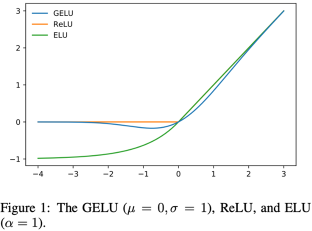
- GELU, which was introduced in this paper, is
where $\xi\sim\mathcal{N}(0, 1)$ and $\Phi$ is the cdf of a standard gaussian distribution.
- **Swish**, introduced in Searching for activation functions, is as follows:
Here, $\beta$ is a parameter and $\sigma$ is the familiar sigmoid function. GELU can be approximated with Swish as $x\sigma(1.702x)$.
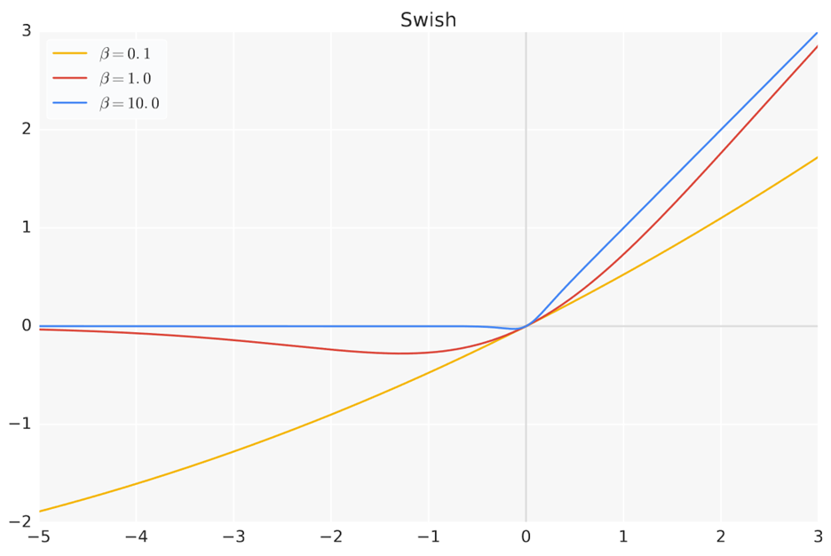
A particular case with $\beta=1$ is known as Sigmoid Linear Unit
\[\mathrm{SiLU}(x) = x\cdot\sigma(x)\]Gated MLP
Probably the most popular FFN architecture today is a GatedMLP. It was introduced under the name of SwiGLU in GLU Variants Improve Transformer. Here’s what it looks like in Qwen2.5-3B-Instruct:
SwiGLU recalls a gating mechanism from LSTMs: it’s like up_proj(x) is the information we’re passing through and SiLU(gate_proj(x)) controls how much of this information we want to pass through the FFN layer. Of course, it’s exactly like that (because SiLU is not $\sigma$), but this may help getting an intuition for it.
On the image above you can also observe a typical dimension patter: the internal dimension of FFN tends to be significantly higher that the input/output dimension. (Also, see Llama 3.1 parameters.)
Normalization
This layer stabilizes training by normalize each token’s hidden‐state vector across its feature dimensions. The original transformer architecture featured the LayerNorm layer, which for a hidden vector $x\in\mathbb{R}^d$ computed
where $\epsilon$ (typically $10^{-6}$) ensures numerical stability, and $\gamma,\beta\in\mathbb{R}^d$ are learned per-feature scale and shift parameters.
RMSNorm
This normalization layer was introduced in Root Mean Square Layer Normalization paper. It ignores centering and simply sets the scale. So, for a vector $x$ the new values will be:
\[\overline{x}_i = \frac{x_i}{\text{RMS}(x_i)}g_i\]In this case, $g_i$ is trainable and the following formula is used to calculate RMS(x):
RMSNorm yields comparable performance against LayerNorm but shows superiority in terms of running speed with a speed-up of $7\%\sim 64\%$; it seems to be the state-of-the-art at present.
Pre-normalization
Pre-normalization was introduced in this paper and it suggests one, performing normalization before attention and before FFN (rather than after them); and two, running normalization in parallel to the residue stream:
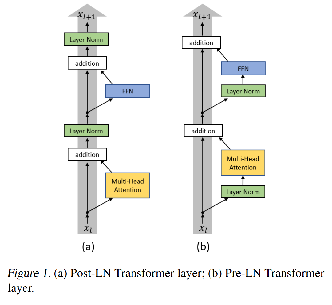
Motivation: the authors of that aforementioned paper show that, with Post-LN, the expected gradients of the parameters near the output layer are large. Therefore, the warm-up stage is needed at the beginning of the training process where the optimization starts with an extremely small learning rate. This is necessary because the optimization process can become unstable otherwise. For more details, check the theoretical analysis in the paper.
Some additional details about attention
Masked attention
There is an important difference between how self-attention is used in encoder-only models (such as BERT) and in LLMs (which are decoder-only models):
- In encoder-only models, each token “attends” to each token.
- In LLMs, a token never ”attends’’ to future tokens. (Indeed, when we’re generating a text, we can’t know what going to be in the future.)
At this point, it’s also good to note that there are, in a sense, two different modes of LLM operation:
- During the autoregressive generation phase, we generate new tokens one by one, and these tokens simply can’t “see” whatever is not yet generated.
- However, during the prompt processing phase, the LLM has access to all the prompt tokens, and the prompt tokens must be deliberately prohibited from “looking” at the later tokens. This might have been implemented by processing the prompt token by token, but this would be very inefficient. Instead, the prompt is processed in one pass with attention masking.
To understand what the attention mask is, let’s recall how self-attention works:
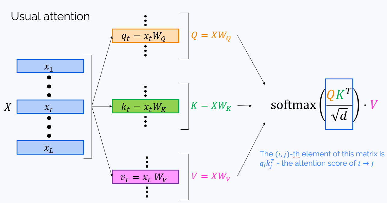
To prevent “looking into the future”, we need to zero all elements of $QK^T$ over the main diagonal (those with $i < j$). This can be done by elementwise multiplication on the $0-1$ matrix called attention mask:
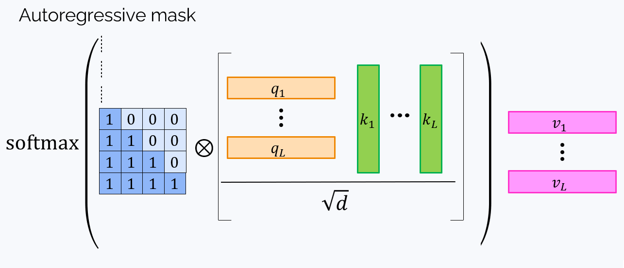
Here, $\otimes$ stands for the elementwise product. The final formula for the attention is as follows:
\[o = \mathbf{softmax}\left(\frac{M\otimes QK^T}{\sqrt{d}}\right)V\]Note: It’s not often mentioned, but in today’s LLMs, the self-attention layer often has one additional operation: $y = oW_o$
Note: In today’s implementations, an elementwise product is often replaced by an elementwise sum with a matrix $M’$ that has $-\infty$ above the diagonal. (The softmax of $-\infty$ is zero, so that also works.)
Some details about attention heads
Despite being described as totally separate layers, in reality, attention heads work as follows:
- Theoretically, each $i$-th attention head has its own matrices: $W_{i,Q},W_{i,K}, W_{i,V}, W_{i,O}$,
-
Yet in practice, they are stored and applied each as one matrix:
\[W_Q = \begin{pmatrix}W_{1,Q} & W_{2,Q} & \cdots & W_{\text{n}\_\text{heads}, Q}\end{pmatrix}\]etc. When applying it, we do
\[q_{total} = xW_Q,\]and after that the row vector $q_{total}$ is cut into $\text{n_heads}$ row vectors $q_1, q_2,\ldots, q_{\text{n_heads}}$.
-
So, for example, if Llama3.1-8B has a model dimension (=hidden size) 4,096 and 32 attention heads, then each attention head’s query has a dimension of $\frac{4096}{32} = 128$.
Note that Llama 3.1 has less key and value heads than it has query heads. This is due to Grouped Query Attention that we’ll discuss below.
A quest for efficient attention
The attention mechanism is at the heart of every transformer, so it’s not surprising that many variations of it emerged since 2017.
The main problem with attention is its quadratic complexity, and indeed, each token must attend to each token. Moreover, standard procedure involves calculating the matrix $QK^T$ (product of matrix of all queries and the matrix of all keys) which can be very large.
The complexity of the attention mechanism is one of the main bottlenecks in the struggle towards large context length, and, as we’ll see, many of the improvements noted below are aimed towards making attention a little more lightweight and efficient.
Sliding window attention
Most likely drawing inspiration from convolutional networks, sliding window attention suggests to consider only a fixed window around each token, thus making the computational cost linear on the context length.

The upper layers receive information from a longer subsequence. As in convolutions, attention window can be dilated to make receptive field wider.
Though sliding window attention is not used in top-tier LLMs, it’s still a popular ingredient in the attempts at making LLMs more efficient with long context.
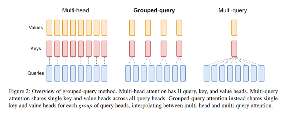
Group query attention
Even a single attention mechanism is costly, and going multi-head only makes it worse. Here’s an idea to mitigate this: have only one attention head for values and keys, and keep many heads for queries. This approach is called multi-query attention, and it’s nice, but very restrictive.
The next step was suggested in GQA: Training Generalized Multi-Query Transformer Models from Multi-Head Checkpoints, that is, having many value heads, which are grouped on several value and key heads:
Now we can return to Llama-3.1.
For the 8B model, the table shows that the number of Key/Value Heads is 8. Given that there are 32 attention heads (=how many queries), we see that there are 4 query heads per key/value. Moreover, with the attention head dimension of 128, we may see that the dimensions of the total $W_Q$ and $W_K$ are $\text{hidden_dim}\times(128\cdot 8) = 4096\times1024$.
Key-Value caches
Key-value caches are now a natural feature of almost every transformer model. They store keys and values (that is $k_i = x_iW_K$ and $v_j = x_jW_V$), allowing us not to recompute them each time we need to generate the next token.
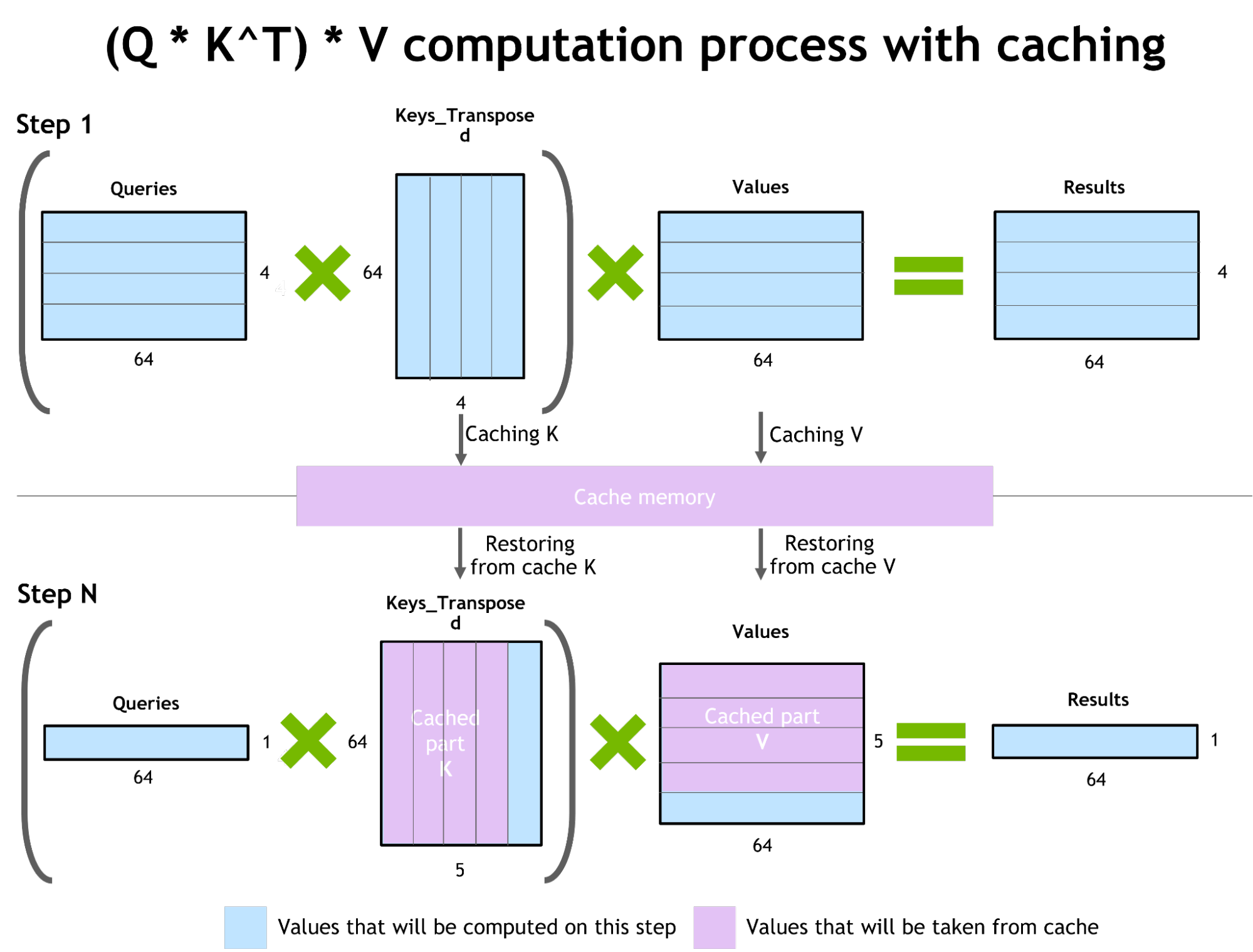
However this approach comes with a drawback of its own: memory consumption. For long sequences, the size of a KV-cache may become comparable with the size of the model itself. This, in turn, motivates researchers to find ways of reducing the size of the KV-cache. This is generally out of this long read’s scope, but we’ll share a couple of references in case if you’re curious:
- Compression along the sequence length
- Compression across the layers
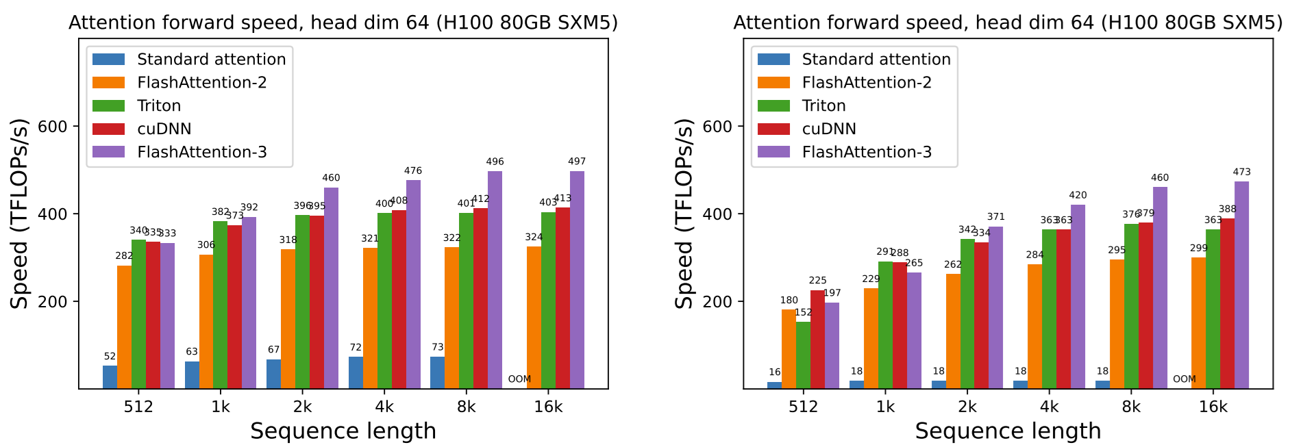
Leveraging the infrastructure: Flash attention
The previous improvements we discussed were hardware-agnostic; now it’s time to briefly discuss how leveraging GPU architecture can help.
Introduced in FlashAttention: Fast and Memory-Efficient Exact Attention with IO-Awareness, FlashAttention, together with its descendants, became a state of the art attention optimization.
Instead of proposing a new attention mechanism, the authors leverage hardware capabilities - in particular the GPU memory hierarcy, which comprises:
- high bandwidth memory (HBM), slower but larger;
- on-chip SRAM, faster but smaller.
As compute has gotten faster relative to memory speed, operations are increasingly bottlenecked by memory (HBM) accesses. Thus, exploiting fast SRAM becomes more important.
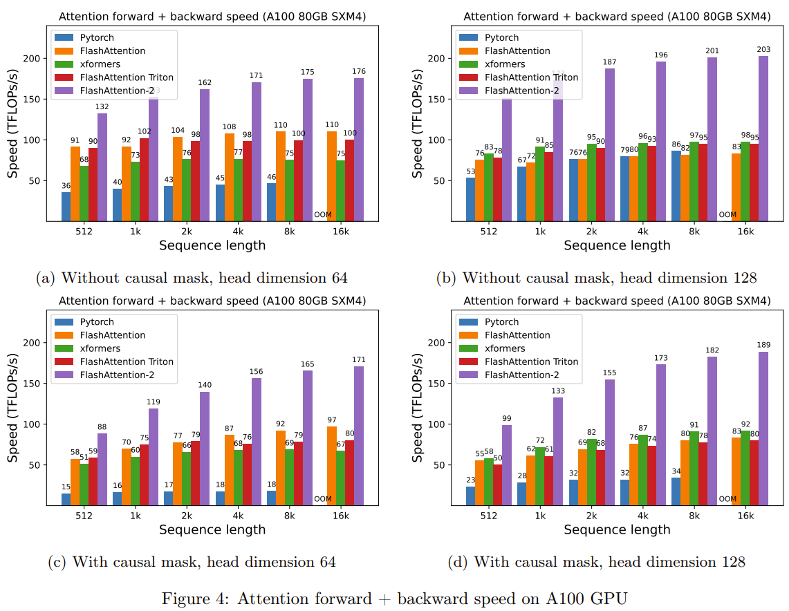
The idea is to fuse the whole attention computation $(Q, K, V)\mapsto\text{softmax}\left[\text{Mask}\left(QK^T/\sqrt{d}\right)\right]V$ into a single tiled GPU kernel, avoiding materializing the full attention matrix. But be aware that it only works on sufficiently advanced GPUs.

Tri Dao, the first author of FlashAttention later published further improvement of this algorithm: \href{https://arxiv.org/pdf/2307.08691.pdf}{FlashAttention-2: Faster Attention with Better Parallelism and Work Partitioning}. It is really efficient and widely used now to the extent that proposing new modifications of attention mechanish is running of out fashion: FlashAttention-2 gives better out-of-the box performance than almost any new attention scheme that doesn’t work with FlashAttention-2.
In July ‘24 Tri Dao and his team published even more efficient \href{https://tridao.me/publications/flash3/flash3.pdf}{FlashAttention-3}, optimized for H100.
FlashAttention and its descendants have several drawbacks as well:
- It doesn’t work with just any GPU;
- Even with the right GPU, you can just fail to make it work on you virtual machine;
- It’s incompatible with some other nice things.
Positional encoding
The non-masked attention mechanism used in encoder-only models is oblivious to token order - every token “attends” to every token, turning the model basically into a clever Bag of Words. To fix that, Positional encoding was suggested.
With LLMs, the problem is not that acute thanks to masked attention. Indeed, the fact that every token only “attends” to itself and the previous ones, introduces some degree of order understanding into the model. That’s why LLMs with a lack of position encoding whatsoever (a mechanism known as NoPE - No Positional Encoding) aren’t totally a failure. Though, even for LLM things are bettwer with some positional encoding. So, let’s discuss the existing mechanisms.
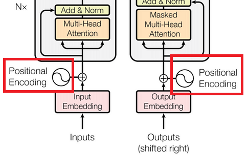
Absolute positional encoding
The original transformer paper suggested using absolute positional encoding: this is a special vector for each position number $i$ that is added to the token embedding.
Relative positional encoding
Relative positional encoding was introduced by Google in Self-Attention with Relative Position Representations.
Motivation: the reasoning to introduce relative positional encoding (as opposed to absolute positional encoding) came about because of the fact that relative positions are more relevant for the attention mechanism than absolute positions.
First of all, let’s change our view on positional embeddings; they are necessary to introduce information about positions into the attention mechanism, so let’s consider them as details inside of this:
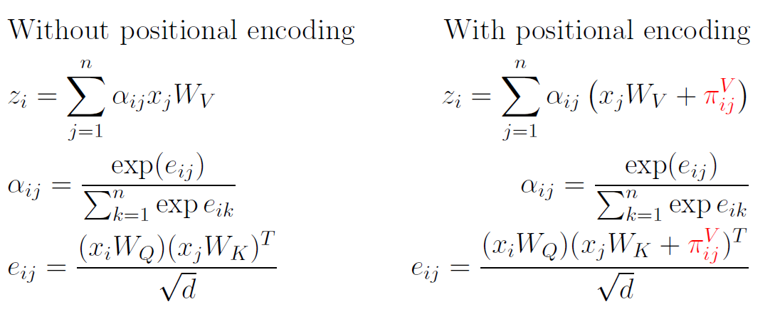
Note that in the original transformer architecture, positional embeddings are indeed introduced into each attention layer due to residual connections. However, in modern architectures, this is no longer equivalent due to pre-normalization.
Now, relative positional encoding suggests to set:
\[\pi_{ij}^K = w^K_{\mathrm{clip}(j - i, k)},\] \[\pi_{ij}^V = w^V_{\mathrm{clip}(j - i, k)}\]Here, $\mathrm{clip}(x, k) = \max(-k, \min(k, x))$ for some fixed clipping distance $k$ (the width of an attention window). The vectors $w^K$ and $w^V$ are learned during the traning of a transformer.
Rotary embeddings (RoPE)
Rotatry embeddings were introduced in the RoFormer paper and have since become the state-of-the-art within the world of position encoding.
Again, with this we consider positional encoding as a way of influencing attention mechanism.
This idea is often formulated in the language of complex numbers, and I’ll explain the concept shortly in the appendix below, but here, I will use the language of matrices instead.
Rotation matrix in 2D. A counterclockwise rotation by angle $\varphi$ around the origin is a linear transformation of the 2D plane $\mathbb{R}^2$, and as such, it can be written using a matrix like so:
\[(x, y)\mapsto (x, y)\cdot\begin{pmatrix} \cos{\varphi} & \sin{\varphi}\\ -\sin{\varphi} & \cos{\varphi} \end{pmatrix}\]However, it’s cumbersome to write this matrix every time we need to rotate something. Luckily, we can use a shortcut:
\[(x, y)\cdot e^{i_\varphi}\text{\mathbf{ is the same as }}(x, y)\cdot\begin{pmatrix} \cos{\varphi} & \sin{\varphi}\\ -\sin{\varphi} & \cos{\varphi} \end{pmatrix}\]I will very briefly explain the math behind $e^{i\varphi}$ in the appendix, but for the purpose of understanding the positional embedding, you can just treat it as a short notation for the rotation matrix.
Now, back to rotary embeddings!
The authors of the RoPE paper drew inspiration from yet another formulation of additive positional encoding for queries and keys:
\[q_m = (x_m + \pi^Q_m)W_Q, \quad k_n = (x_n + \pi^K_n)W_K\]But instead of using the ready formulas, they want to substitute the right parts with some new functions:
\[q_m = f_q(x_m, m),\quad k_n = f_k(x_n, n)\]Here, $q_mk^T_n$ only depends on the relative position of $m - n$ (and not on $m$ and $n$ themselves).
For 2-dimensional $x_i$, $k_i$, $q_i$ the authors mathematically proved that $f_q$ and $f_k$ should be of the following form:
\[f_q(x_m, m) = x_mW_Qe^{im\theta},\quad f_k(x_n, n) = x_nW_Ke^{in\theta}.\]Indeed, in this case it is:
\[f_q(x_m, m)\cdot f_k(x_n, n)^T =\] \[=x_mW_Q\begin{pmatrix} \cos{m\theta} & \sin{m\theta}\\ -\sin{m\theta} & \cos{m\theta} \end{pmatrix}\cdot\begin{pmatrix} \cos{n\theta} & -\sin{n\theta}\\ \sin{n\theta} & \cos{n\theta} \end{pmatrix}W_K^Tx_n^T =\] \[x_mW_Qe^{i(m-n)\theta}W_K^Tx_n^T\]For the arbitrary dimension $d$ (which we assume to be an even number) we use a block-diagonal rotation matrix:
\[f_q(x_m, m) = x_mW_QR^d_{\Theta, m},\quad f_k(x_n, n) = x_nW_KR^d_{\Theta, n},\]where
\[R^d_{\Theta, m} = \begin{pmatrix} \cos{m\theta_1} & \sin{m\theta_1} & 0 & 0 & \dots & 0 & 0\\ -\sin{m\theta_1} & \cos{m\theta_1} & 0 & 0 & \dots & 0 & 0\\ 0 & 0 & \cos{m\theta_2} & \sin{m\theta_2} & \dots & 0 & 0\\ 0 & 0 & -\sin{m\theta_2} & \cos{m\theta_2} & \dots & 0 & 0\\ \vdots & \vdots & \vdots & \vdots & \ddots & \vdots & \vdots\\ 0 & 0 & 0 & 0 & \dots & \cos{m\theta_{d/2}} & \sin{m\theta_{d/2}}\\ 0 & 0 & 0 & 0 & \dots & -\sin{m\theta_{d/2}} & \cos{m\theta_{d/2}}\\ \end{pmatrix},\]….where the parameters $\Theta$ are set to this:
\[\theta_i = 10000^{-2(i-1)/d}\]But be cautious! If you read through the original paper, you’ll find that everything is multiplied in inverse order; for example, $f_q(x_m, m) = R^d_{\Theta, m}W_Qx_m$. The matrix $R^d_{\Theta, m}$ also appears to be transposed. This ambiguity is due to the fact that the ML community can never agree on the answer to a simple question: are $x_i$ row vectors or column vectors? In our interpretation $x_i$ are rows, so they get multiplied from the right. But the authors of the RoPE paper see x_i as columns, so all the multipliers go to the left.
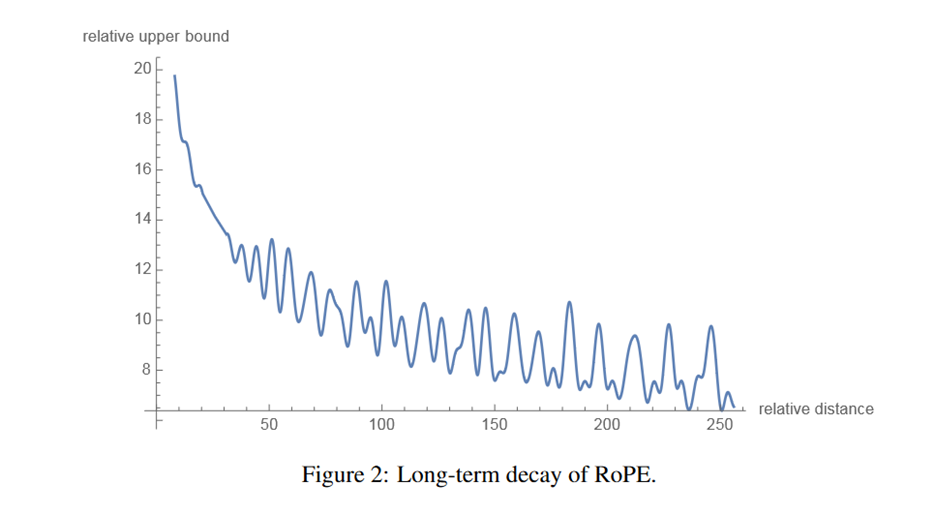
Long-term decay. RoPE embeddings provide long-term decay property, which means the $q_mk_n^T$ will decay when the relative position increases. Take this illustration from the paper:
Linearized attention
Actually, in the RoPE paper, the attention mechanism’s formulation is a bit peculiar, and it is inspired by the Transformers are RNNs paper. Let’s dive into it. The typical mechanism that operates with queries $q_n$, keys $k_n$ and values $v_n$ transforms values as follows:
\[v_n' = \frac{\sum_{m=1}^N\mathrm{sim}(q_n, k_m)v_m}{\sum_{m=1}^N\mathrm{sim}(q_n, k_m)}\qquad(\ast)\]Here, $\mathrm{sim}$ is a similarity function of sorts, for example, $\mathrm{sim}(q_n, k_m) = \exp\left(\frac{q_mk_n^T}{\sqrt{d}}\right)$. Indeed, the traditional
\[v_n' = \sum_{m=1}^N\frac{\exp\left(\frac{q_mk_n^T}{\sqrt{d}}\right)}{\sum_{m=1}^N\exp\left(\frac{q_mk_n^T}{\sqrt{d}}\right)}v_m,\]can be rewritten exactly like $(\ast)$.
The authors of “Transformers are RNNs” observe that we can choose different similarity functions as long as they are positive. They suggest taking
\[\mathrm{sim}(q_n, k_m) = \psi(q_n)\phi(k_m)^T\]for some functions $\psi, \phi$. In particular, they propose $\psi(x) = \phi(x) = \mathrm{ELU}(x) + 1$, where
\[\mathrm{ELU}(x) = \begin{cases} x, &x > 0\\ a(e^x - 1), &x\leqslant 0 \end{cases}\]The authors of RoPE suggest taking the formula
\[v_n' = \sum_{m=1}^N\frac{\psi(q_n)\phi(k_m)^T}{\sum_{m=1}^N\psi(q_n)\phi(k_m)^T}v_m,\]and plugging in RoPE as follows:
\[v_n' = \sum_{m=1}^N\frac{\left(\psi(q_n)R^d_{\Theta, n}\right)\left(\phi(k_m)R^d_{\Theta, m}\right)^T}{\sum_{m=1}^N\psi(q_n)\phi(k_m)^T}v_m,\]Note that there are no RoPEs in the denominator (to avoid it becoming zero), so the numbers
\[\frac{\left(\psi(q_n)R^d_{\Theta, n}\right)\left(\phi(k_m)R^d_{\Theta, m}\right)^T}{\sum_{m=1}^N\psi(q_n)\phi(k_m)^T}, m=1,\ldots,N\]no longer give a probabilistic distribution — but the authors claim that it’s all right anyway.
RoPE and long context
Today’s LLMs have quite generous context lengths, like 128k, or 200k, or even 1M+. But they aren’t pre-trained for 200k from the start! Indeed, training on long sequences is very taxing, so LLMs are usually pre-trained with progressive context length, like
- First on sequences up to 8,192 tokens (and that may be the largest training bulk)
- Then on sequences up to 16,384 tokens
- Finally, after 3-5 stages like this, you arrive to the target 200k or 1M
But now, there’s a problem. Imagine that you’ve only trained your model on sequences of length $\leqslant8192$, so that that during the training it has only seen RoPE matrices with $0\leqslant m,n\leqslant8192$. It won’t suddenly generalize for larger $m,n$. If you try to feed a longer sequence to such a model, you should expect poor results. So, you need to somehow extrapolate RoPE outside its comfortable range. Let’s discuss how it is done.
Position interpolation
One of the first solutions to this problem was suggested in this paper: Extending context window of large language models via position interpolation. The idea was that if we want to move from max context length $L$ to max context length $L’$, we can just shrink the new range $[0, L’]$ to the old one $[0, L]$. So, we thus change this: $f_q(x_m, m) = x_mW_QR^d_{\Theta, m},\quad f_k(x_n, n) = x_nW_KR^d_{\Theta, n},$ Into this: $f’{q,k}(x_m, m) = f{q,k}\left(x_m, \frac{mL}{L’}\right)$
This picture demonstrates extrapolation (upper) vs. interpolation (lower):
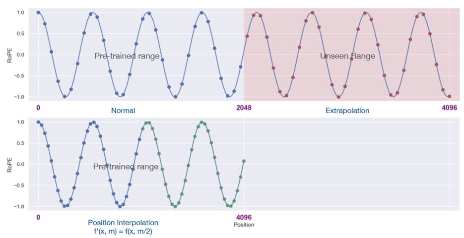
Why is it called interpolation? Instead of extrapolating $f(x_m, m)$ outside of the comfortable $[0, L]$ we need to interpolate it for non-integer values $\frac{mL}{L’}$. Experiments show that this works better.
The “NTK-aware” method
First of all, let’s write a generalized form of RoPE. We had $f_{q,k}(x_m, m, \Theta) = x_mW_{Q,K}R^d_{\Theta, m}$, where $\theta_j = b^{-2j/d}$ with base $b = 10000$.
Now let’s write $f_{q,k}(x_m, g(m), h(\Theta))$, where $g$ and $h$ can be some functions.
For ordinary position interpolation we have $g(m) = \frac{m}{s},\quad h(\Theta) = \Theta,$ where $s = \frac{L’}{L}$. .
What can be a problem with interpolation?
In ordinary attention we’ll have the $e^{-i(n-m)\theta}$ term in $f_{q}(x_n, n, \Theta)f_{k}(x_m, m, \Theta)^T$ which, after interpolation, becomes $e^{-i(n/s-m/s)\theta}$, and for large $s$ and small $n-m$ the term $\frac{n-m}{s}$ may become too small. So, interpolated positions can do a bad job with close tokens, and since close tokens usually have strong ties, this can severely decrease quality.
There are several ways of mitigating this.
Base change. The authors of Code LLaMA suggest instead of scaling the range increasing base $b$ from 10,000 to 1,000,000 for fine-tuning.
The “NTK-aware” method is a base change with a particular new base value:
$g(m) = m,
h(\theta_j) = (b’)^{-2j/d},$
where $b’ = b\cdot s^{\frac{d}{d-2}}$.
Note that NTK-aware method combines both interpolation and extrapolation.
The YaRN paper uses an elaborate version of this, treating different coordinates (different $j$) in a different way, depending on the wavelength of RoPE, which is defined as $\lambda_j = \frac{2\pi}{\theta_j} = 2\pi b^{2j/p}$. The idea is as follows:
- If the wavelength $\lambda_j$ is much smaller than the context size $L$, we do not interpolate
- If the wavelength $\lambda_j$ is equal to or bigger than the context size $L$, we want to only interpolate and avoid any extrapolation (unlike the previous “NTK-aware” method)
- Dimensions in-between can have a bit of both, similar to the “NTK-aware” interpolation
We’ll skip the formulas, but you can check them in the YaRN paper.
But what is “NTK”? NTK stands for Neural Tangent Kernels, and NTK-aware interpolation has an interesting mathematical interpretation, which we’ll unfortunately skip here. If you’re curious about it, you can check this paper: Fourier Features Let Networks Learn High Frequency Functions in Low Dimensional Domains.
Mixture of experts
The Mixture of Experts (MoE) approach was first brought to LLMs with the Mixtral model. It had its own ups and downs in the LLM history; recent models that use MoE include DeepSeek-V3 (and its descendant DeepSeek-R1) and two models from the Qwen3 family: Qwen3-30B-A3B and Qwen3-235B-A22B.
We really recommend browsing the blog post Mixture of Experts Explained blog post to better understand its inner workings and to get a feel on how to make it really efficient.
Mixtral has a similar architecture to Mistral 7B, but some of the Feedforward layers are replaced with a sparse MoE (Mixture of Experts) layer.
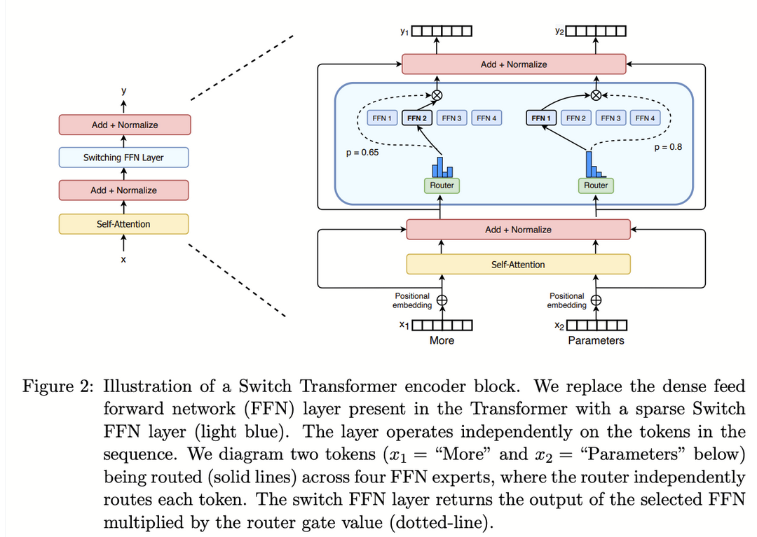
Here’s what we have here: a gating function that decides which expert will receive the input $x$. It works as follows.
-
First, for each expert number $i$ it calculates
\[H(x)_i = {(x\cdot W_g)}_{i} + \text{StandardNormal()}\cdot\text{SoftPlus}((x\cdot W_{noise})_i),\]where $W$’s are trainable weigths and randomness aids load balancing.
-
Then, we only pick experts with top $k$ values of $H$:
\[\mathrm{KeepTopK}(H(x), k)_i = \begin{cases} H(x)_i, &\text{if $H(x)_i$ is among the top-$k$ of $H(x)_i$},\\ -\infty, &\text{otherwise}. \end{cases},\] -
And finally:
\[G(x) = \mathrm{softmax}(\mathrm{KeepTopK}(H(x), k))\] -
Now, the output is calculated as follows::
\[y = \sum_iG(x)_iE_i(x)\]Note that only $k$ experts $E_i$ are employed each time
For example, Qwen3-235B-A22B has 128 experts, with only 8 of those activated for each token. (This information may be checked in its model card.)
Why does this matter? If we compare Mistral to Mixtral, we see two things:
- Mixtral has a much larger number of total parameters: 46.7B as opposed to Mistral’s 7B. So, accordingly, you’ll need more memory to store it — but at the same time, the model is potentially much more powerful than Mistral.
- That said, on inference time you don’t use all the parameters because out of many experts you only employ several (for example, $2$). In the case of Mixtral, only 12.9B parameters are used for each inference call. This makes the model almost as quick as Mistral, while also being much more powerful.
For example, the name Qwen3-235B-A22B means that the model has 235B parameters in total, with only 22B activated for each token.
There are many more interesting features to explore with this approach; for example, load balancing. Dealing with experts is worth it if you can parallelize their jobs, but depending on gating, some of them may remain underemployed, thus severely limiting overall efficiency. The authors use some interesting ideas to deal with this; check the paper to explore this further.
Appendix: complex numbers
On several occasions while discussing rotary embeddings we encountered the expression $e^{i\varphi}$. To understand what it really means, let’s venture briefly in the world of complex numbers.
In essence, a complex number is something of form $a + bi$, where $i$ is a phantom number satisfying $i^2 = -1$. There are several good things about complex numbers:
-
The sum of two complex numbers is a complex number:
\[(a_1 + b_1i) + (a_2 + b_2i) = (a_1 + a_2) + (b_1 + b_2)i\] -
Complex numbers have a convenient interpretation as vectors of a two-dimensional plane:
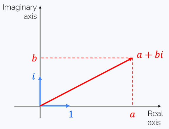
And the sum of two complex numbers = the sum of their corresponding vectors.
-
The product of two complex numbers is, again, a complex number:
-
Euler’s formula: $e^{i\varphi} = \cos{\varphi} + i\sin{\varphi}$. If you want to check this, just write Taylor’s expansions of exponent, sine and cosine and use the fact that $i^2 = -1$, $i^3 = -i$, $i^4 = 1$, etc.
-
Multiplication by $e^{i\varphi}$ rotates a vector by angle $\varphi$ (counterclockwise if $\varphi > 0$):
…which is indeed the result of the rotation of $z = (a, b)$ by angle $\varphi$.